Page 134 - Distributed model predictive control for plant-wide systems

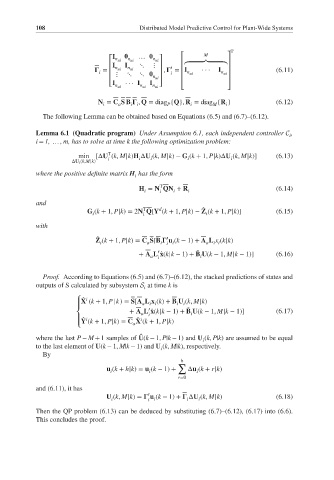
108 Distributed Model Predictive Control for Plant-Wide Systems

T
I … ⎡ M ⎤
⎡ n ui n ui n ui ⎤ ⏞⏞⏞⏞⏞⏞⏞⏞⏞⏞⏞⏞⏞⏞⏞⏞⏞
⎢I I ⋱ ⋮ ⎥ ′ ⎢ ⎥
n ui
= ⎢ n ui ⋱ ⋱ ⎥ , = I n ui ··· I n ui ⎥ (6.11)
⎢
⋮
i
i
⎢ n ui⎥ ⎢ ⎥
⎣I ··· I I ⎦ ⎢ ⎥
n ui n ui n ui ⎣ ⎦
N = C S B , Q = diag {Q}, R = diag {R } (6.12)
M
i
i
i
a
i i
P
The following Lemma can be obtained based on Equations (6.5) and (6.7)–(6.12).
Lemma 6.1 (Quadratic program) Under Assumption 6.1, each independent controller C ,
i
i = 1, … , m, has to solve at time k the following optimization problem:
T
min [ΔU (k, M|k)H ΔU (k, M|k)− G (k + 1, P|k)ΔU (k, M|k)] (6.13)
i
i
i
i
ΔU i (k,M|k) i
where the positive definite matrix H has the form
i
T
H = N QN + R (6.14)
i i i i
and
d
T
G (k + 1, P|k)= 2N Q[Y (k + 1, P|k)− Z (k + 1, P|k)] (6.15)
̂
i i i
with
′
̂
Z (k + 1, P|k)= C S[B u (k − 1)+ A L x (k|k)
i a i i i a i i
′
+ A L ̂ x(k|k − 1)+ B U(k − 1, M|k − 1)] (6.16)
̃
i
a i
Proof. According to Equations (6.5) and (6.7)–(6.12), the stacked predictions of states and
outputs of S calculated by subsystem S at time k is
i
⎧ ̂ i a i i i i
X (k + 1, P |k) = S[A L x (k)+ B U (k, M|k)
⎪ ′
̃
+ A L ̂ x(k|k − 1)+ B U(k − 1, M|k − 1)] (6.17)
⎨ a i i
⎪ ̂ i ̂ i
Y (k + 1, P|k)= C X (k + 1, P|k)
⎩ a
where the last P − M + 1 samples of Û(k − 1, P|k − 1) and U (k, P|k) are assumed to be equal
i
to the last element of U(k − 1, M|k − 1) and U (k, M|k), respectively.
i
By
h
∑
u (k + h|k)= u (k − 1)+ Δu (k + r|k)
i i i
r=0
and (6.11), it has
′
U (k, M|k)= u (k − 1)+ ΔU (k, M|k) (6.18)
i i
i
i
i
Then the QP problem (6.13) can be deduced by substituting (6.7)–(6.12), (6.17) into (6.6).
This concludes the proof.