Page 157 - Distributed model predictive control for plant-wide systems

Networked Distributed Predictive Control with Information Structure Constraints 131

⎡ ⎤
∑
⎢ C x (k) ⎥
i 1 j j
⎢ ⎥
, j∉j∈P −i ,
⌢
j∈P +i 1
v (k)= ⎢ ⋮ ⎥ (7.14)
i
⎢ ⎥
∑
C x (k)
⎢ ⎥
i n j j
⎢ ⎥
, j∉j∈P −i ,
⎣ j∈P +i n ⎦
It should be noticed that the input of this neighborhood model is still the input of S , and the
i
inputs of S ∈ P , j ≠ i are regarded as disturbances. It is because each local MPC can only
j
−i
determine the manipulated variables of the corresponding subsystem.
Due to the unit delay introduced by the network (see Assumption 1), the information of other
subsystems is available only after one sampling time interval. Therefore, controller C uses
i
⌢
⌢
̂
̂
w (k + l − s|k − 1)) and v (k + l|k − 1) computed on the basis of information related to time
i
i
k − 1 to estimate the interactions, and the initial states of downstream neighbors are substituted
T
with ̂ x (k|k − 1)(h = 1, … , n).For i = 1, … , m, define
i h
[ ] T
T
T
⌢ T ̂ x (k|k − 1) · · · ̂ x (k|k − 1)
x (k|k)= x (k |k) i 1 i n (7.15)
i
i
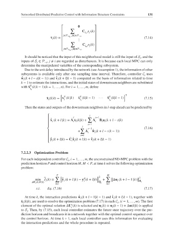
Then the states and outputs of the downstream neighbors in l-step ahead can be predicted by
l
⎧
⌢ l ∑ ⌢ s−1 ⌢
x (k + l |k) = A x (k|k)+ A B u (k + l − s|k)
⎪ ̂ ⌢ ⌢
i i i i i i
⎪
s=1
⎪ l
∑ ⌢ s−1 (7.16)
⎨ ⌢ ̂
+ A i w (k + l − s|k − 1))
i
⎪
s=1
⎪
⌢
⌢
⌢
⌢
̂
̂
⎪ ̂ y (k + l|k)= C x (k + l|k)+ v (k + l|k − 1)
i
i i
i
⎩
7.2.2.3 Optimization Problem
For each independent controller C , i = 1, … , m, the unconstrained ND-MPC problem with the
i
prediction horizon P and control horizon M, M < P,attime k solves the following optimization
problem:
P M
∑ d 2 ∑ 2
min J (k)= ‖ ⌢ ̂ i ‖ ‖ Δu (k + l − 1 |k) ‖
‖y (k + l |k) − y (k + l|k)‖ ⌢ +
i
i
ΔU i (k,M|k) ‖ i ‖Q i ‖ ‖R i
l=1 l=1
s.t. Eq. (7.16) (7.17)
⌢
⌢
At time k, the interaction predictions w (k + l − 1|k − 1) and v (k + l|k − 1), together with
̂
̂
i i
⌢
x (k|k), are used to resolve the optimization problem (7.17) in each C ,(i = 1, … , m). The first
i i
∗
element of the optimal solution ΔU (k) is selected and u (k)= u (k − 1)+Δu(k|k) is applied
i i i
to S . Then, by (7.15), each local controller estimates the future state trajectory over the pre-
i
diction horizon and broadcasts it in a network together with the optimal control sequence over
the control horizon. At time k + 1, each local controller uses this information for evaluating
the interaction predictions and the whole procedure is repeated.