Page 159 - Distributed model predictive control for plant-wide systems

Networked Distributed Predictive Control with Information Structure Constraints 133

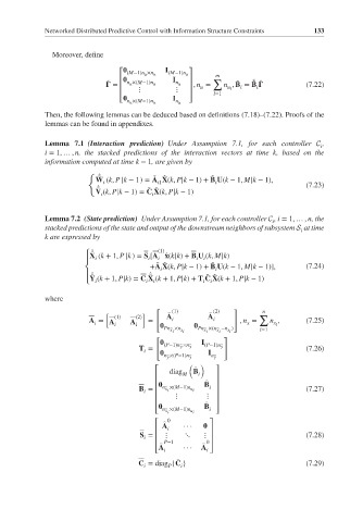
Moreover, define
I
⎡ (M−1)n u ×n u (M−1)n u ⎤ m
⎢ I ⎥ ∑
̃ ̃ ̃
̃
= n u ×(M−1)n u n u , n = n , B = B (7.22)
̃
⎢ ⋮ ⋮ ⎥ u u l i i
⎢ ⎥ l=1
⎣ I
n u ×(M−1)n u n u ⎦
Then, the following lemmas can be deduced based on definitions (7.18)–(7.22). Proofs of the
lemmas can be found in appendixes.
Lemma 7.1 (Interaction prediction) Under Assumption 7.1, for each controller C ,
i
i = 1, … , n, the stacked predictions of the interaction vectors at time k, based on the
information computed at time k − 1, are given by
{
⌢ ̂
̂
̃
̃
W (k, P |k − 1) = A X(k, P|k − 1)+ B U(k − 1, M|k − 1),
i
i
i1
⌢ ̂ (7.23)
̃ ̂
V (k, P|k − 1)= C X(k, P|k − 1)
i
i
Lemma 7.2 (State prediction) Under Assumption 7.1, for each controller C ,i = 1, … , n, the
i
stacked predictions of the state and output of the downstream neighbors of subsystem S at time
i
k are expressed by
⎧ ̂ ⌢ (1)
X (k + 1, P |k) = S [A ̂ x(k|k)+ B U (k, M|k)
i
i
i
i
i
⎪
̃ ̂
̃
+A X(k, P|k − 1)+ B U(k − 1, M|k − 1)], (7.24)
⎨ i i
⎪ ̂ ⌢ ⌢ ̂ ̃ ̂
⎩ Y (k + 1, P|k)= C X (k + 1, P|k)+ T C X(k + 1, P|k − 1)
i
i
i
i
i
where
[ ] n
[ ] ⌢ (1) ⌢ (2) ∑
(1) (2) A A
A = A = i i , n = n , (7.25)
i i A i x x l
Pn ⌢ ×n x i Pn ⌢ ×(n ⌢ −n x i ) l=1
x i
x i
x i
[ ]
I
y
T = (P−1)n ⌢ ×n ⌢ y (P−1)n ⌢ y (7.26)
i
⌢ ×(P−1)n ⌢ I ⌢
n y y n y
( )
⌢
diag M B i
⎡ ⎤
⎢ ⎥
⌢
B ⎥
i
B = n x i (7.27)
⎢ ⌢ ×(M−1)n u i
i
⎢
⋮ ⎥
⎢ ⋮ ⎥
⌢
⎢ B ⎥
x i
⎣ n ⌢ ×(M−1)n u i i ⎦
⌢ 0
⎡ ⎤
A i ···
⎢ ⎥
S = ⎢ ⋮ ⋱ ⋮ ⎥ (7.28)
i
⎢ ⌢ P−1 ⌢ 0 ⎥
⎣A i ··· A ⎦
i
⌢
C = diag {C } (7.29)
i P i