Page 162 - Distributed model predictive control for plant-wide systems

136 Distributed Model Predictive Control for Plant-Wide Systems

is rewritten into the following form:
[ ]
m P M
∑ ∑ d 2 ∑ 2
min ‖ i ‖ + ‖ Δu (k + l − 1 |k) ‖
‖̂ y (k + l |k) − y (k + l|k)‖
i
ΔU i (k,M|k) ‖ i ‖Q i ‖ ‖R i
i=1 l=1 l=1
̂ x (k + l + 1 |k) A A ··· A ̂ x (k + l |k)
⎡ i ⎤ ⎡ ii ii 1 ii n ⎤ ⎡ i ⎤
⎢A
⎢̂ x (k + l + 1|k)⎥ i 1 i A ··· A ⎥ ⎢̂ x (k + l|k)⎥
s.t. i 1 = i 1 i 1 i n i n i 1
⎢ ⋮ ⎥ ⎢ ⋮ ⋮ ⋱ ⋮ ⎥ ⎢ ⋮ ⎥
⎢ ⎥ ⎢ ⎥ ⎢ ⎥
⎣̂ x (k + l + 1|k)⎦ ⎣A i n i A ··· A ⎦ ⎣̂ x (k + l|k)⎦
i n i n i 1 i n i n i n
B (7.39)
⎡ ii ⎤
i 1 i
⎢B ⎥
⌢
+ u (k + l|k)+ w (k + l|k − 1))
̂
⎢ ⋮ ⎥ i i
⎢ ⎥
⎣B ⎦
i n i
̂ x (k + l + 1|k)= ̂ x (k + l + 1|k − 1), (j ∉ P )
j j −i
̂ y (k + l|k)= C ̂ x (k + l|k)+ ̂ v (k + l|k − 1), (i = 1, … , m)
i i i i
Δu (k + l − 1|k)=Δu (k + l − 1|k − 1), (j ≠ i)
j j
If using the local performance index (7.4), as in [46], for each controller C , i = 1, … , m,the
i
optimization problem of the distributed MPC can be written in the following form:
[ ]
m P M
∑ ∑ d 2 ∑ 2
min ‖ j ‖ + ‖ j ‖
‖̂ y (k + l |k) − y (k + l|k)‖
‖Δu (k + l − 1 |k)‖
ΔU i (k,M|k) ‖ j ‖Q j ‖ ‖R j
j=1 l=1 l=1
s.t. ̂ x (k + l + 1|k)= A x (k + l|k)+ B u (k + l|k)+ ̂ w (k + l|k − 1));
ii i
ii i
i
i
⌢
⌢
̂ y (k + l|k)= C ̂x (k + l|k)+ v (k + l|k − 1)
̂
i i i i
̂ y (k + l|k)= ̂ y (k + l|k − 1) (j ≠ i)
j j
Δu (k + l − 1|k)=Δu (k + l − 1|k − 1)(j ≠ i) (7.40)
j j
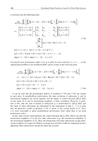
It can be seen that the performance indices of problems (7.39) and (7.40) are similar
to each other. In neighborhood optimization, the state evolutions of subsystem S and its
i
downstream neighbors are solved together, and the impact of control decision ΔU (k, M|k)
i
on the states of S and its downstream neighbors is fully considered. However, in prob-
i
lem (7.40), only the state evolution of subsystem S is determined by ΔU (k, M|k) and
i i
the states of other subsystems are substituted by the estimations at time k − 1. It is clear
that the predictive model in problem (7.39) is closer to the system model (5.3). Thus,
it is more reasonable to adopt neighborhood performance index rather than to use local
performance index.
In fact, after several control periods, the control decision ΔU (k, M|k) affects not only the
i
downstream neighbors of S but also other subsystems (e.g., the downstream neighbors of
i
the downstream neighbors of S ). Here, the interactions with other subsystems except down-
i
stream neighbors are neglected. If there is enough network band-width for employing iterative
algorithm, these interactions can also be taken into account.