Page 161 - Distributed model predictive control for plant-wide systems

Networked Distributed Predictive Control with Information Structure Constraints 135

Remark 7.1 The resulting complexity to obtain the closed-form solution for the local
subsystem S is mainly given by the inversion of matrix H . Considering that the size of
i
i
3
3
matrix H equals M ⋅ n , the complexity of the inversion algorithm is O(M , n ) if using the
i u i u i
Gauss–Jordan algorithm. Therefore, the total computational complexity of the distributed
( )
∑ n
3 3
solution is O M , n , while the computational complexity of the centralized MPC is
i=1 u i
( )
( ) 3
3 ∑ n
O M , n .
i=1 u i
7.2.4 Stability Analysis
On the basis of the closed-form solution stated in Theorem 7.1, the closed-loop dynamics can
be specified and the stability condition can be verified by analyzing the closed-loop dynamic
matrix. Thus, the following theorem is obtained.
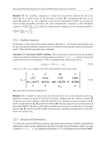
Theorem 7.2 (Networked DMPC stability) The closed-loop system given by the feedback
connection of plant S with the set of independent controller C ,i = 1, … , n, whose closed-form
i
control laws are given by Equation (7.36), is asymptotically stable if and only if
| {A }| < 1, ∀j = 1, … , n N (7.37)
j
N
where n = Pn + n + 2Mn is the order of the global closed-loop system.
x
N
x
u
A
⎡ B ⎤
⎢ ⎥
⎢ LSA LSB ⎥
LS A LS B
̃
̃
A = ⎢ ⎥ (7.38)
N
̃ ⎥
̃
A + LS A
⎢ LSA B + LS B + LSB
⎢ ⎥
⎢ I ⎥
⎣ Mn u ⎦
The proof can be found in Appendix. E.
Remark 7.2 It should be noticed that the first two block rows of the dynamic matrix A
N
depend on element of matrix A (the first two block columns) and the element of matrix B
(in the last two block columns), while the third block row depends on process matrices A, B,
and C, weight matrices Q , R and horizons P and M. This fact suggests a key for the design of
i i
networked-DMPC. The degree of freedom available to the designer is on the choices of weight
matrices Q , R , and horizons P and M, which introduce significant modifications on the third
i i
block row of matrix A .
N
7.2.5 Analysis of Performance
To explain the essential differences between the optimization problem with the neighborhood
optimization index and the optimization problem with the local performance index, for each
controller C , i = 1, … , n, the optimization problem (7.17) of the proposed networked DMPC
i