Page 164 - Distributed model predictive control for plant-wide systems

138 Distributed Model Predictive Control for Plant-Wide Systems

d d
Temperatur y n-1 y d n
y d y 1 y 2 y 3 d y 4 d Desired cooling curve
d

O l 1 l 2 l 3 l 4 L l i-1 l i L l n-1 l n Position l
Heat flow Plate thickness
Entry
energy Δz Exit
flow Δl Γ energy
flow
S 1 S 2 S 3 S 4
Open dynamic system Γ S n-1 S n
Finishing Mill Leveller
TP1 TP2 Laminar cooling headers TP3 TP4

1 2 3 4 5 6 7 8 9 10 1112131415
A B C

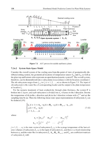
Figure 7.1 ACC process for middle and heavy plates
7.2.6.2 System State-Space Model

Consider the overall system of the cooling area from the point of view of geometrically dis-
tributed setting system, the geometrical locations of temperature sensor T P2 and T P3 as well as
the plate top and bottom sides represent an open thermodynamic system . The overall system,
therefore, can be dismembered into n subsystems in accordance with the location coordinate l.
The sth subsystem ranges from l s−1 to l (s = 1, 2, … , m) as shown in Figure 7.5. The input of
s
sth subsystem is the water flux of corresponding header and the output is the plate temperature
at location l .
s
For the numeric treatment of heat conductivity through plate thickness, the system is
broken into L layers, and each subsystem is divided into n volumes in the l-direction. Denote
s
the temperature of ith in the z-direction and jth in the l-direction volume with x (i, j) and set the
s
sampling time be Δt. Then the following linear state-space representation of subsystem S can
s
be deduced [19]:
⎧ x (k + 1) = A ⋅ x (k)+ B ⋅ u (k)+ D ⋅ x (k)
s ss s ss s s,s−1 s−1
⎪
⎨ y (k)= C ⋅ x (k) (7.42)
ss
s
s
⎪ s = 1, 2, … , m
⎩
where
[ T T T ] T
x = (x ) (x ) ··· (x s,n s )
s,2
s
s,1
[ ] T
(1, j) (2, j) (L, j)
x = x x ··· x
s, j s s s
j = 1, 2, … , n is the state vector of subsystem S , y is the average temperature of the last col-
s s s
umn volumes of subsystem S , u is the input of subsystem S , and there is a fixed relationship
s s s
between u and the water flux in subsystem S . A , B , D , and C are coefficient matrices
s s ss ss s,s−1 ss
of subsystem S with
s