Page 175 - Distributed model predictive control for plant-wide systems

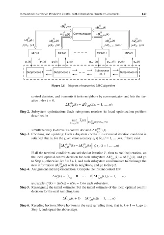
Networked Distributed Predictive Control with Information Structure Constraints 149

(l)
∆U 1,M (k) (l)
∆U m,M (k)
(l) (l)
∆U 2,M (k) Communicator ∆U m–1,M (k)
(l) (l) (l) (l)
∆U j,M (k) ∆U j,M (k) ∆U j,M (k) ∆U j,M (k)
j∈¥ 1 , j≠1 j∈¥ 2 , j≠2 j∈¥ m–1 , j≠m–1 j∈¥ m , j≠m

MPC1 MPC2 MPCm-1 MPCm

u 1 (k) y 1 (k) u 2 (k) y 2 (k) u m-1 (k) y m–1 (k) u m (k) y m (k)

Subprocess
Subprocess 1 Subprocess 2 Subprocess m
m–1

Figure 7.8 Diagram of networked MPC algorithm

control decision, and transmits it to its neighbors by communicator, and lets the iter-
ative index l = 0:
(l)
̂
ΔU (k)=ΔU (k)(i = 1, … , m)
i,M i,M
Step 2. Subsystem optimization: Each subsystem resolves its local optimization problem
described in
|
min J (k) | (l)
i
ΔU i,M (k) | ΔU j,M (k)(j∈ℕ i , j≠i)
|
(l+1)
simultaneously to derive its control decision ΔU (k).
i,M
Step 3. Checking and updating: Each subsystem checks if its terminal iteration condition is
satisfied, that is, for the given error accuracy ∈ ℝ, (i = 1, … , m), if there exist
i
‖ (l+1) (l) ‖
‖ΔU i,M (k)−ΔU i,M (k)‖ ≤ , (i = 1, … , m)
i
‖ ‖
∗
If all the terminal conditions are satisfied at iteration l , then to end the iteration, set
∗
the local optimal control decision for each subsystem ΔU ∗ (k)=ΔU (l ) (k), and go
i,M i,M
to Step 4; otherwise, let l = l + 1, and each subsystem communicate to exchange the
(l)
new information ΔU (k) with its neighbors, and go to Step 2.
i,M
Step 4. Assignment and implementation: Compute the instant control law
[ ] ∗
∗
Δu (k)= I ··· ΔU (k), (i = 1, … , m)
i n ui i,M
∗
∗
∗
and apply u (k)=Δu (k)+ u (k − 1) to each subsystem.
i i i
Step 5. Reassigning the initial estimate: Set the initial estimate of the local optimal control
decision for the next sampling time
̂
ΔU (k + 1)=ΔU ∗ (k)(i = 1, … , m)
i,M i,M
Step 6. Receding horizon: Move horizon to the next sampling time, that is, k + 1 → k,goto
Step 1, and repeat the above steps.