Page 170 - Distributed model predictive control for plant-wide systems

144 Distributed Model Predictive Control for Plant-Wide Systems

7.3 Networked DMPC with Iterative Algorithm
In the previous section, we introduced a networked DMPC for a distributed system. As has
been mentioned before, the closed-loop system will achieve “Nash optimality” if the iterative
algorithm is employed in the LCO-DMPC and the closed-loop system could obtain “Pareto
optimality” if the iterative algorithm is employed in the global cost optimization-based DMPC.
The iteration could indeed improve the global performance of the closed-loop system in the
distributed control framework. Thus, in this section, we will develop the networked DMPC
with an iterative algorithm. In the procedure of resolving the optimal problem, each subsystem
only communicates with its neighbors, which is rather easy to fulfill the network requirements.

7.3.1 Problem Description

n
n
Consider a distributed system composed of m subsystems, where y ∈ ℝ n and u ∈ ℝ i are the
i i
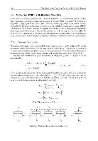
output and manipulated vectors for the subsystem S , respectively. This system is composed
i
of many similar subsystems placed after one another, in such a way that each subsystem is
connected with dynamic control input coupled with its neighbor subsystems (Figure 7.6).
The input interacted the state-space model of each subsystem S , refer to Chapter 4, can be
i
represented by
∑
⎧
x (k + 1) = A x (k)+ B Δu (k)
i
j
i i
ij
⎪
j∈P i (i = 1, … , m) (7.43)
⎨
⎪y (k)= C x (k)
i i i
⎩
where Δu (k) is the increment of the manipulated variable (or control decision) at the time
i
T
instant k, u(k)=Δu (k)+ u(k − 1), x(k)=[x (k) ··· x (k)] ∈ ℝ n y i is the state vector of the
T
T
i i1 iN
subsystem S , P called the neighborhood of the subsystem i , which includes the upstream
i
i
neighbors and the downstream neighbors of S , and with
i
[ ]
I
A = (N−1)n yi ×n yi (N−1)n yi
i
n yi ×(N−1)n yi I n yi
[ ] T
T
T
B = a (1) ··· a (N)
ij ij ij
[ ]
C = I n yi n yi ×(N−1)n yi
i
k−1
C A B = a (k), k = 1, 2, …
i i ij ij
u 1 u i−1 u i u i+1 u m
Subprocess Subprocess Subprocess Subprocess Subprocess
1 i-1 i i+1 m
y 1 y i−1 y i y i+1 y m
Figure 7.6 Diagram of a serially connected process