Page 171 - Distributed model predictive control for plant-wide systems

Networked Distributed Predictive Control with Information Structure Constraints 145

{C , A } is observable, a (k)(k = 1, … , N; j ∈ P ) is the sampled output matrix array of the
i
ij
i
i
subsystem S for the subsystem S unit step input at the sampling time instant k, N is the
i
j
modeling horizon. It can be seen that the output of each subsystem is dependent on control
inputs of its own and its neighbor subsystems. It can be seen that the state-space model
described in Equation (7.43) for each subsystem is developed directly from step responses
without further identification. It is not necessary to identify the structure of the subsystem
during the modeling. The optimization and/or control strategy can be employed with the
usual state-space techniques.
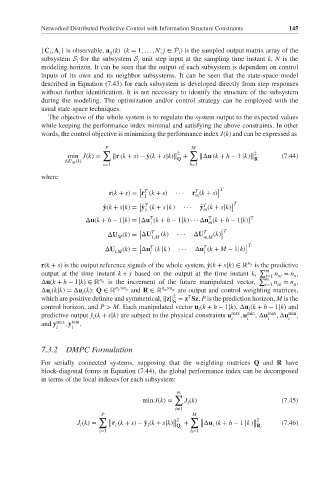
The objective of the whole system is to regulate the system output to the expected values
while keeping the performance index minimal and satisfying the above constraints. In other
words, the control objective is minimizing the performance index J(k) and can be expressed as
P M
∑ 2 ∑ 2
min J(k)= ‖r (k + s) − ̂ y(k + s|k)‖ + ‖Δu (k + h − 1 |k)‖ (7.44)
ΔU M (k) Q R
s=1 h=1
where

[ T T ] T
r(k + s)= r (k + s) ··· r (k + s)
1 m
[ T T ] T
̂ y(k + s|k)= ̂ y (k + s |k) ··· ̂ y (k + s|k)
m
1
T
T
Δu(k + h − 1|k)=[Δu (k + h − 1|k) ··· Δu (k + h − 1|k)] T
1 m
[ T T ] T
ΔU (k)= ΔU 1,M (k) ··· ΔU m,M (k)
M
[ T T ] T
ΔU i,M (k)= Δu (k |k) ··· Δu (k + M − 1|k)
i
i
n y
r(k + s) is the output reference signals of the whole system, ̂ y(k + s|k)∈ ℝ is the predictive
∑ m
output at the time instant k + s based on the output at the time instant k, i=1 yi y
n = n ,
Δu(k + h − 1|k)∈ ℝ n u is the increment of the future manipulated vector, ∑ m n = n ,
u
i=1 ui
Δu (k|k)=Δu (k); Q ∈ ℝ n y ×n y and R ∈ ℝ n u ×n u are output and control weighting matrices,
i
i
2
T
which are positive definite and symmetrical, ‖z‖ = z Sz, P is the prediction horizon, M is the
S
control horizon, and P > M. Each manipulated vector u (k + h − 1|k), Δu (k + h − 1|k) and
i
i
predictive output ̂y (k + s|k) are subject to the physical constraints u max , u min , Δu max , Δu min ,
i
i
i
i
i
and y max , y min .
i i
7.3.2 DMPC Formulation
For serially connected systems, supposing that the weighting matrices Q and R have
block-diagonal forms in Equation (7.44), the global performance index can be decomposed
in terms of the local indexes for each subsystem:
m
∑
min J(k)= J (k) (7.45)
i
i=1
P M
∑ 2 ∑ 2
J (k)= ‖ r (k + s) − ̂ y (k + s|k) ‖ + ‖ Δu (k + h − 1 |k) ‖ (7.46)
i ‖ i i ‖Q i ‖ i ‖R i
s=1 h=1