Page 189 - Distributed model predictive control for plant-wide systems

Networked Distributed Predictive Control with Information Structure Constraints 163

T = diag{T , … , T }
1 n
= diag{ K , … , K } (E.10)
1
n
n
1
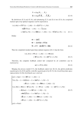
By definitions (E.5) and (E.10), and substituting (E.3) and (E.4) into (E.9), the completed
stacked open-loop optimal sequence can be expressed as
d
(k, M|k)= (k − 1, M|k − 1)+ {Y (k + 1, P|k)
′ ̂
′
− S[B (k − 1, M|k − 1)+ Âx(k|k)
+ A (k, P|k − 1)+ B (k − 1, M|k − 1)] − TC (k, P|k − 1)} (E.11)
̃
̂
̃
̂
̃
Define
=− SA
̃
=− (SA + TC )
̃
′
′
= − S(B + B ) (E.12)
̃
Then the completed stacked open-loop optimal sequence (D.11) has the form
(k, M|k)= (k − 1, M|k − 1)+ ̂x(k|k)
d
̂
+ (k, P|k − 1)+ Y (k + 1, P|k) (E.13)
Therefore, the complete feedback control law computed by all controllers can be
expressed as
u(k)= U(k, M|k) (E.14)

Merging the process model (5.3), the feedback control law (E.14), the global prediction
equation given by (E.8) and the controller equation given by (E.13), the closed-loop state-space
representation for the distributed case is derived

⎧x(k)= Ax(k − 1)+ B (k − 1, M|k − 1)
⎪
⎪ ̂ ̃ ̂
(k, P|k − 1)= LS[Âx(k − 1)+ A (k − 1, P|k − 2)
⎪
⎪ ̃
+ B (k − 1, M|k − 1)+ B v(k − 2, M|k − 2)]
⎪
⎪ d
(k, M|k)= ̂x(k)+ (k, P|k − 1)+ (k − 1, M|k − 1)+ Y (k + 1, P|k)
̂
⎪
⎪
= [Ax(k − 1)+ B (k − 1, M|k − 1)] (E.15)
⎨
⎪
̃
+ LS[Âx(k − 1)+ A (k − 1, P|k − 2)
̂
⎪
⎪
̃
⎪ +B (k − 1, M|k − 1)+ B (k − 2, M|k − 2)]
⎪
d
⎪ + (k − 1, M|k − 1)+ Y (k + 1, P|k)
⎪
⎪ y(k)= Cx(k)
⎩