Page 190 - Distributed model predictive control for plant-wide systems

164 Distributed Model Predictive Control for Plant-Wide Systems

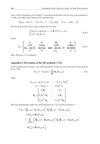
where ̂x(k|k) in Equations (E.8) and (E.13) has been substituted with x(k) due to the assumption
of fully accessible state. Defining the extended state
[ T ] T
̂ T
̂ T
̂ T
X (k)= x (k) (k, P|k − 1) (k, M|k) (k − 1, M|k − 1) ,
N
the closed-loop state-space representation has the form
{
d
X (k) = A X (k − 1)+ B Y (k + 1, p|k)
N N N N
(E.16)
y(k)= C X (k)
N
N
where
A B
⎡ ⎤
⎢ LSA LSB ⎥
̃
LS A LS B
̃
A = ⎢ ⎥ (E.17)
N
̃
⎢ A + LS A LSA B + LS B + LSB ⎥
̃
⎢ I ⎥
⎣ Mn u ⎦
Thus, Theorem 7.2 is obtained.
Appendix F. Derivation of the QP problem (7.52)
At the sampling time instant k, the output prediction model for each subsystem can be derived
from (7.48)
∑
Y (k)= G ̂ x (k)+ H ΔU (k) (F.1)
̂
i,P i i ij j,M
j∈ℕ i
where
[ T T ] T
Y (k)= ̂ y (k + 1 |k) · · · ̂ y (k + P|k)
̂
i,P i i
[ T P T ]
G = (C A ) ··· (C A )
i
i
i
i
i
C B ···
⎡ ⎤
i ij
⎢ ⋮ ⋱ ⋮ ⎥
⎢ M−1 ⎥
H = C A B ··· C B
ij ⎢ i i ij i ij ⎥
⎢ ⋮ ⋮ ⋮ ⎥
⎢ C A P−1 B ··· C A P−M B ⎥
⎣ i i ij i i ij⎦
The local performance index for each subsystem in (7.51) can be rewritten as
[ ] T [ ]
J (k)= R (k) − H ΔU (k) Q R (k) − H ΔU (k)
i i,P ii i,M i i,P ii i,M
+ΔU T (k)R ΔU (k)
i,M i i,M
{
∑ [ ] T [ ]
+ R (k) − H ΔU (k) Q R (k) − H ΔU (k)
j,P ji i,M j j,P ji i,M
j∈P i , j≠i
}
+ΔU T (k) R ΔU (k)
j,M j j,M