Page 187 - Distributed model predictive control for plant-wide systems

Networked Distributed Predictive Control with Information Structure Constraints 161

is used together with Equations (7.24) and (7.30) to obtain the output prediction in the form
⌢ ̂
̂
Y (k + 1, P|k)= N ΔU (k, M|k)+ Z(k + 1, P|k). By substituting this expression, the local
i i i
cost function J takes the form (7.31). The positive definiteness of matrices Q and R implies
i
i
i
the same property for matrix H .
i
In this way, the ND-MPC problem has been transformed into an equivalent unconstrained
QP problem which has to be locally solved online at each sampling instant.
Appendix D. Proof of Theorem 7.1
States that a solution to the ND-MPC problem minimizes the cost function (7.31) with
respect to the control sequence ΔU (k, M|k). This solution has the form ΔU (k, M|k)=
i i
−1
((1∕2)H G (k + 1, P|k)). Following the receding horizon strategy, only the first element of
i i
the optimal sequence is actually applied to the process and the control action is expressed as
u (k)= u (k − 1)+ ΔU (k, M|k) which gives the final closed form (7.36).
i i i i

Appendix E. Proof of Theorem 7.2
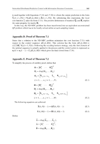
To simplify the process of stability proof, define that

= T ··· T ] T
[
1 P
= diag{ , … , }
j
nj
1j
[ ]
= I
ij n x i ×(j−1)n x i n x i n x i ×(P−j)n x i
(i = 1, … , n, j = 1, … , P); (E.1)
[
= T ··· T ] T
1 M
= diag{ , … , }
j 1j nj
[ ]
= I
ij n u i ×(j−1)n u i n u i n u i ×(M−j)n u i
(i = 1, … , n, j = 1, … , M) (E.2)
The following equations are achieved
̂
X(k, P|k − 1)= ̂ X(k, P|k − 1) (E.3)
U(k, M|k − 1)= U(k, M|k − 1) (E.4)

Define

A = diag{A , … , A };
11
n1
[ ] T
̃ T
̃ T
A = A ··· A n ;
̃
1
B = diag{B , … , B };
1
n