Page 201 - Distributed model predictive control for plant-wide systems

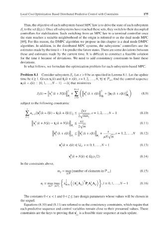
Local Cost Optimization Based Distributed Predictive Control with Constraints 175

Thus, the objective of each subsystem-based MPC law is to drive the state of each subsystem
S to the set Ω ( ). Once all subsystems have reached these sets, they switch to their decoupled
i i
controllers for stabilization. Such switching from an MPC law to a terminal controller once
the state reaches a suitable neighborhood of the origin is referred to as the dual mode MPC
[69]. For this reason, the DMPC algorithm we propose in this chapter is a dual mode DMPC
algorithm. In addition, in the distributed MPC systems, the subsystems’ controllers use the
estimates made by the time k − 1 to predict the future states. There are some deviations between
these and estimates made by the current time. It is difficult to construct a feasible solution
for the time k because of deviations. We need to add consistency constraints to limit these
deviations.
In what follows, we formulate the optimization problem for each subsystem-based MPC.
Problem 8.1 Consider subsystem S .Let > 0 be as specified in Lemma 8.1. Let the update
i
time be k ≥ 1. Given x (k) and ̂ x (k + s|k), s = 1, 2, … , N, ∀j ∈ P , find the control sequence
i j +i
u (k + s|k)∶{0, 1, … , N − 1} → U that minimizes
i
i
N−1 ( )
2 ∑ 2
‖ p ‖ ‖ p ‖ 2
J (k)= ‖x (k + N|k)‖ + + u (k + s|k) ‖ (8.9)
‖
i ‖ i ‖x (k + s|k)‖ ‖ i ‖R i
‖ i
‖P i
s=0 ‖Q i
subject to the following constraints:
s
∑
p
||x (k + l|k)− ̂ x (k + l|k)|| ≤ √ , s = 1, 2, … , N − 1 (8.10)
s−l i i 2
l=1 2 mm 1
‖ p ‖
i
‖x (k + N|k) − ̂ x (k + N|k)‖ ≤ √ (8.11)
‖ i ‖P i 2 m
‖ p ‖ ‖ f ‖
‖x (k + s|k)‖ ≤ ‖x (k + s|k)‖ + √ , s = 1, 2, … , N (8.12)
‖ i ‖P i ‖ i ‖P i
N m
p
u (k + s|k)∈ U , s = 0, 1, … , N − 1 (8.13)
i i
p
x (k + N|k)∈Ω ( ∕2) (8.14)
i i
In the constraints above,
m =max{number of elements in P } (8.15)
2 +i
i∈P
{ }
1 ( )
( l ) T l
2
=max max max A A ij P A A ij , l = 0, 1, … , N − 1 (8.16)
j
l
ii
ii
i∈P j∈P i
The constants 0 < < 1 and 0 < ≤ 1are design parameters whose values will be chosen in
the sequel.
Equations (8.10) and (8.11) are referred to as the consistency constraints, which require that
each predictive sequence and control variables remain close to their presumed values. These
f
constraints are the keys to proving that x is a feasible state sequence at each update.
j,i