Page 86 - Distributed model predictive control for plant-wide systems

60 Distributed Model Predictive Control for Plant-Wide Systems

To derive (4.25), we note that
( )
y i
y = Gu ⇒ = Element(G, i, j)
u
j u k =0,k≠j
Interchange the roles of G and G − 1 ,the rolesof u and y, and the roles of subscribe i and j,
it yields [83]
( )
u j
−1
−1
u = G y ⇒ = Element(G , j, i)
y
i y k =0,k≠i
and (4.25) follows. Reference [86] points out that the ratio between the gains in (4.24) and
(4.25) is a useful measure of interactions between the jth input and the ith output, and defines
the relative gain of the jth input to the ith output as
ij
g ij
−1
≜ = Element(G, i, j) ⋅ Element(G , j, i) (4.26)
ij
g
̂
ij
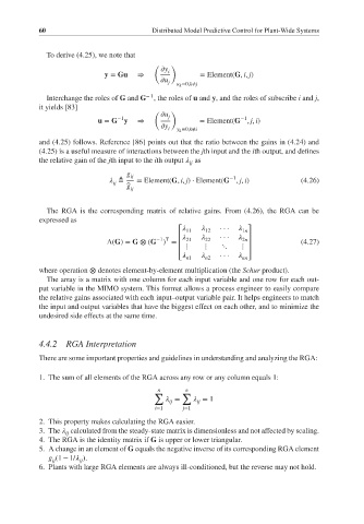
The RGA is the corresponding matrix of relative gains. From (4.26), the RGA can be
expressed as
⎡ 11 12 ··· ⎤
1n
2n
−1 T
Λ(G)= G ⊗ (G ) = ⎢ 21 22 ··· ⎥ (4.27)
⎢ ⋮ ⋮ ⋱ ⋮ ⎥
⎢ ⎥
⎣ n1 n2 ··· ⎦
nn
where operation ⊗ denotes element-by-element multiplication (the Schur product).
The array is a matrix with one column for each input variable and one row for each out-
put variable in the MIMO system. This format allows a process engineer to easily compare
the relative gains associated with each input–output variable pair. It helps engineers to match
the input and output variables that have the biggest effect on each other, and to minimize the
undesired side effects at the same time.

4.4.2 RGA Interpretation
There are some important properties and guidelines in understanding and analyzing the RGA:

1. The sum of all elements of the RGA across any row or any column equals 1:
n n
∑ ∑
= = 1
ij ij
i=1 j=1
2. This property makes calculating the RGA easier.
3. The calculated from the steady-state matrix is dimensionless and not affected by scaling.
ij
4. The RGA is the identity matrix if G is upper or lower triangular.
5. A change in an element of G equals the negative inverse of its corresponding RGA element
g (1 − 1/ ).
ij
ij
6. Plants with large RGA elements are always ill-conditioned, but the reverse may not hold.