Page 88 - Distributed model predictive control for plant-wide systems

62 Distributed Model Predictive Control for Plant-Wide Systems

PC

LB

x D
u 1
u 0

u 2
LB
x B

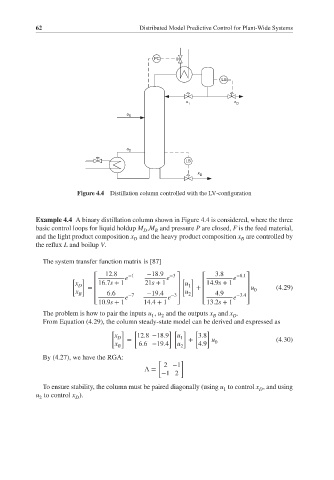
Figure 4.4 Distillation column controlled with the LV-configuration

Example 4.4 A binary distillation column shown in Figure 4.4 is considered, where the three
basic control loops for liquid holdup M ,M and pressure P are closed, F is the feed material,
D B
and the light product composition x and the heavy product composition x are controlled by
D B
the reflux L and boilup V.
The system transfer function matrix is [87]

12.8 −1 −18.9 3.8
⎡ e e −3 ⎤ ⎡ e −8.1⎤
[ ] [ ]
x D = ⎢16.7s + 1 21s + 1 ⎥ u 1 + ⎢14.9s + 1 ⎥ u (4.29)
x B ⎢ 6.6 −19.4 ⎥ u 2 ⎢ 4.9 ⎥ 0
⎢ e −7 e −3⎥ ⎢ e −3.4⎥
10.9s + 1 14.4 + 1 13.2s + 1
⎣ ⎦ ⎣ ⎦
The problem is how to pair the inputs u , u and the outputs x and x .
1 2 B D
From Equation (4.29), the column steady-state model can be derived and expressed as
[ ] [ ][ ] [ ]
x D = 12.8 −18.9 u 1 + 3.8 u (4.30)
x B 6.6 −19.4 u 2 4.9 0
By (4.27), we have the RGA:
[ ]
2 −1
Λ=
−12
To ensure stability, the column must be paired diagonally (using u to control x , and using
1
D
u to control x ).
D
2