Page 84 - Distributed model predictive control for plant-wide systems

58 Distributed Model Predictive Control for Plant-Wide Systems

In this theorem, the first condition points out that the inputs could be able to affect all the
states. The second condition points out that the degree of freedom of inputs is large enough to
regulate the state to the desired value.

Example 4.2 Judge the structure controllability of the structured system (A, B) expressed by
(4.15) and (4.16).

First, let us check the input accessibility according to condition (1) in Theorem 4.2. From
Example 4.1, the system (A, B) is input accessible.
Then what we need to do is to check the generic rank of [A, B], according to condition (2)
in Theorem 4.2
0 0 ∗ ∗ 0 ∗ 0 0 0
⎡ ⎤
⎢0 0 ∗ 0 ∗ 0 0 ∗
[ ] ∗⎥
A B = 0 0 ∗ ∗ 0 0 0 0 ∗ ⎥ (4.22)
⎢
⎢ ⎥
0 0 ∗ ∗ 0 ∗ ∗ 0 0
⎢ ⎥
⎣0 0 ∗ 0 0 ∗ 0 0 ∗⎦
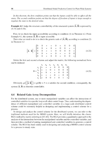
Delete the first and second columns and adjust the matrix; the following normalized form
can be deduced:
x 3 x 4 x 1 x 4 u 2 u 5 u 3
x ∗ ∗ ∗ 0 0 0 0
1 ⎡ ⎤
x 3 ⎢∗ ∗ 0 ∗ 0 0 0⎥
S = (4.23)
x 5 ⎢ ∗ 0 ∗ ∗ 0 0 0 ⎥
x ⎢ ∗ ∗ ∗ 0 ∗ 0 0 ⎥
4 ⎢ ⎥
x 2 ⎣∗ 0 0 ∗ 0 ∗ ∗⎦
([ ])
Obviously, gr A B = gr(S]) = 5 = n satisfies the second condition; consequently, the
system (A, B) is structure controllable.

4.4 Related Gain Array Decomposition
For the distributed system, one or more manipulated variables can affect the interactions of
controlled variables in a specific loop or all other control loops. Thus, understanding the depen-
dence of different manipulated and controlled variables in a large-scale distributed control
scheme could be extremely helpful in designing and implementing a control scheme for a
process.
To design and analyze the control scheme for the distributed system, we can refer to the
traditional methods used for the MIMO system. Here, we will briefly introduce the classic
RGA method by mainly referring to [83–85]. The RGA provides a quantitative approach to the
analysis of the interactions between the manipulated variables and the controlled variables, and
then provides a method of pairing manipulated and controlled variables to generate a control
scheme. The RGA has been widely used in designing and analyzing a MIMO control scheme
for a process in steady state.