Page 80 - Distributed model predictive control for plant-wide systems

54 Distributed Model Predictive Control for Plant-Wide Systems

For example, consider the dynamic system

⎧⎡ x (k + 1) ⎤ ⎡ 0.1 0.2 0 ⎤ ⎡ x (k) ⎤ ⎡ 1 0 ⎤ [ ]
1
1
⎪⎢ ⎥ ⎢ ⎥ ⎢ ⎥ ⎢ ⎥ u (k)
1
2
2
⎪⎢ x (k + 1) ⎥ = 0.2 0.5 0.2 ⎥ ⎢ x (k) ⎥ + 0 1 ⎥
⎢
⎢
u (k)
⎪⎢ x (k + 1) ⎥ ⎢ 0 0.2 0.1 ⎥ ⎢ x (k) ⎥ ⎢ 0 0 ⎥ 2
⎣ 3 ⎦ ⎣ ⎦ ⎣ 3 ⎦ ⎣ ⎦
⎪
⎨
⎪[ ] [ ] ⎡ x (k) ⎤
⎪ y (k) 1 0 1
1 0 ⎢ ⎥
2
⎪ = ⎢ x (k) ⎥
y (k) 0 0 1
⎪ 2 ⎢ x (k) ⎥
⎣ 3
⎩ ⎦
We have
⎡∗ ∗ 0⎤ ⎡∗ 0⎤ [ ]
∗ 0 0
A = ∗ ∗ ∗ ⎥ B = 0 ∗ ⎥ C =
⎢
⎢
⎢ ⎥ ⎢ ⎥ 0 0 ∗
⎣ 0 ∗ ∗ ⎦ ⎣ 0 0 ⎦
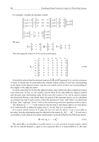
Then the adjacent matrix of (4.9) can be expressed as
x 1 x 2 x 3 u 1 u 2 y 1 y 2
x 1 ⎡∗ ∗ 0 0 0 ∗ 0⎤
x ⎢∗ ∗ ∗ 0 0 0 0⎥
2
x 3 ⎢ 0 ∗ ∗ 0 0 0 ∗ ⎥
A = ⎢ ⎥ (4.10)
a
u
1 ⎢ ∗ 0 0 0 0 0 0 ⎥
u 2 ⎢0 ∗ 0 0 0 0 0⎥
y 1 ⎢ 0 0 0 0 0 0 0 ⎥
⎢ ⎥
y 2 ⎣0 0 0 0 0 0 0⎦
It should be noticed that the structure matrices A, B, and C appeared in A are the transposes
a
of them. It should also be noticed that the columns which consist of zeros are corresponding
to the inputs in the adjacent matrix, and the rows which consist of zeros are corresponding to
the outputs in the adjacent matrix.
It can be seen from (4.10) that the adjacent matrix only reflects the direct impaction among
each subsystem. In fact, we are usually concern about if one unit indirectly impacts another
unit through some intermediate units. In this case, the k power of A can be used to express
a
the interaction during k step ahead. Here, the power of the structure matrix can be calculated
according to the rule of matrix power, where the operation of “plus” and “times” are substituted
by logic “plus” and logic “times” (refer to the maximizing-minimum operation in fuzzy logic).
(k) k
The element a = “ ∗ ”in A expresses that the unit S will impact unit S at k step ahead.
ij a i j
If S could directly or indirectly impact unit S , we say that S is accessible to S .
i j i j
In a system which consists of N units, for any two units S and S , if one is accessible to
i j
2
the other, then the relationship must be reflected in the matrix A , A , … , A N−1 . If each unit is
a
a
a
accessible to itself, then all accessible relationships can be described by the following matrix:
R = I ∪ A ∪···∪ A N−1 (4.11)
a a
The matrix R is so-called the accessible matrix. It is also a kind of structure matrix, where
the ith row and jth element r equal to zero expresses that S is unaccessible to S . By logic
j
ij
i