Page 78 - Distributed model predictive control for plant-wide systems

52 Distributed Model Predictive Control for Plant-Wide Systems

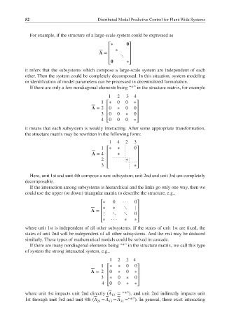
For example, if the structure of a large-scale system could be expressed as
⎡∗ ⎤
⎢ ∗ ⎥
A =
⎢ ⋱ ⎥
⎣ ∗⎦ ⎥
⎢
it refers that the subsystems which compose a large-scale system are independent of each
other. Then the system could be completely decomposed. In this situation, system modeling
or identification of model parameters can be processed in decentralized formulation.
If there are only a few nondiagonal elements being “*” in the structure matrix, for example
1 2 3 4
1 ⎡∗ 0 0 ∗⎤
A = 2 ⎢0 ∗ 0 0⎥
3 ⎢ 0 0 ∗ 0 ⎥
⎢ ⎥
4 ⎣0 0 0 ∗⎦
it means that each subsystem is weakly interacting. After some appropriate transformation,
the structure matrix may be rewritten in the following form:
1 4 2 3
1 ∗ ∗ 0
A = 4 ∗
2 ∗
3 ∗

Here, unit 1st and unit 4th compose a new subsystem; unit 2nd and unit 3rd are completely
decomposable.
If the interaction among subsystems is hierarchical and the links go only one way, then we
could use the upper (or down) triangular matrix to describe the structure, e.g.,
⎡∗ 0 ··· 0⎤
⎢∗ ∗ ⋱ ⋮⎥
A =
⎢ ⋮ ⋱ ⋱ 0 ⎥
⎢ ⎥
⎣∗ · · · ∗ ∗⎦
where unit 1st is independent of all other subsystems. If the states of unit 1st are fixed, the
states of unit 2nd will be independent of all other subsystems. And the rest may be deduced
similarly. These types of mathematical models could be solved in cascade.
If there are many nondiagonal elements being “*” in the structure matrix, we call this type
of system the strong interacted system, e.g.,
1 2 3 4
1 ⎡∗ ∗ 0 0⎤
A = 2 ⎢0 ∗ 0 ∗⎥
3 ⎢ ∗ 0 ∗ 0 ⎥
⎢ ⎥
4 ⎣0 0 ∗ ∗⎦
where unit 1st impacts unit 2nd directly (A = “*”), and unit 2nd indirectly impacts unit
12
1st through unit 3rd and unit 4th (A = A = A =“*”). In general, there exist interacting
31
43
24