Page 74 - Distributed model predictive control for plant-wide systems

48 Distributed Model Predictive Control for Plant-Wide Systems

4.2 System Mathematic Model
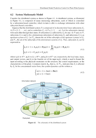
Consider the distributed system as shown in Figure 4.1. A distributed system, as illustrated
in Figure 4.1, is composed of many interacting subsystems, each of which is controlled
by a subsystem-based controller, which in turn is able to exchange information with other
subsystem-based controllers.
Suppose that the distributed system S is composed of m discrete-time linear subsystems S ,
i
i ∈ P = {1, 2, … , m}, and m controllers C , i ∈ P = {1, 2, … , m}. Let the subsystems interact
i
with each other through their states. If subsystem S is affected by S , for any i ∈ P and j ∈ P,
j
i
subsystem S is said to be a downstream subsystem of subsystem S , and subsystem S is an
i j j
upstream system of S .Let P denote the set of the subscripts of the upstream systems of S ,
i +i i
and P the set of the subscripts of the downstream systems of S . Then, subsystem S can be
−i i i
expressed as
∑
⎧
x (k + 1) = A x (k)+ B u (k)+ (A x (k)+ B u (k))
i
ij j
ii i
ii i
ij j
⎪ u
j∈P (4.1)
⎨ i
⎪ y (k + 1)= C x (k)+ C x (k)
ij j
ii i
i
⎩
where x (k)∈ ℝ , u (k)∈ U ⊂ ℝ , and y (k)∈ ℝ n yi are, respectively, the local state, input,
n xi
n ui
i i i i
and output vectors, and U is the feasible set of the input u (k), which is used to bound the
i i
input according to the physical constraints on the actuators, the control requirements, or the
characteristics of the plant. A nonzero matrix A , that is, j ∈ P , indicates that S is affected
ij +i i
by S . In the concatenated vector form, the system dynamics can be written as
j
{
x (k + 1) = Ax(k)+ Bu(k)
(4.2)
y(k + 1)= Cx(k)
Information network
C C 4
C m
C 1
C m-1
C *
C 2
C 3
S 4
S m
S 1
S S m-1
S *
S 2
S 3
Field plant
Figure 4.1 The schematic of the distributed system