Page 76 - Distributed model predictive control for plant-wide systems

50 Distributed Model Predictive Control for Plant-Wide Systems

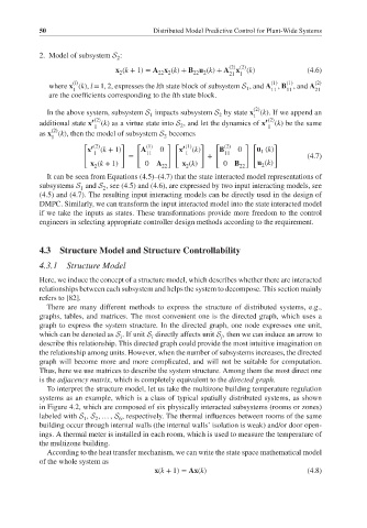
2. Model of subsystem S :
2
(2) (2)
x (k + 1)= A x (k)+ B u (k)+ A x (k) (4.6)
22 2
22 2
2
21 1
(l) (1) (1) (2)
where x (k), l = 1, 2, expresses the lth state block of subsystem S , and A , B , and A
1
1 11 11 21
are the coefficients corresponding to the lth state block.
(2)
In the above system, subsystem S impacts subsystem S by state x (k). If we append an
1 2 1
additional state x ′ (2) (k) as a virtue state into S , and let the dynamics of x ′ (2) (k) be the same
1 2 1
(2)
as x (k), then the model of subsystem S becomes
2
1
[ ′ (2) ] [ (1) ][ ′ (1) ] [ (2) ][ ]
x (k + 1) A 0 x (k) B 0 u (k)
1
1 11 1 11
= + (4.7)
x (k + 1) 0 A 22 x (k) 0 B 22 u (k)
2
2
2
It can be seen from Equations (4.5)–(4.7) that the state interacted model representations of
subsystems S and S , see (4.5) and (4.6), are expressed by two input interacting models, see
2
1
(4.5) and (4.7). The resulting input interacting models can be directly used in the design of
DMPC. Similarly, we can transform the input interacted model into the state interacted model
if we take the inputs as states. These transformations provide more freedom to the control
engineers in selecting appropriate controller design methods according to the requirement.
4.3 Structure Model and Structure Controllability
4.3.1 Structure Model
Here, we induce the concept of a structure model, which describes whether there are interacted
relationships between each subsystem and helps the system to decompose. This section mainly
refers to [82].
There are many different methods to express the structure of distributed systems, e.g.,
graphs, tables, and matrices. The most convenient one is the directed graph, which uses a
graph to express the system structure. In the directed graph, one node expresses one unit,
which can be denoted as S . If unit S directly affects unit S , then we can induce an arrow to
i i j
describe this relationship. This directed graph could provide the most intuitive imagination on
the relationship among units. However, when the number of subsystems increases, the directed
graph will become more and more complicated, and will not be suitable for computation.
Thus, here we use matrices to describe the system structure. Among them the most direct one
is the adjacency matrix, which is completely equivalent to the directed graph.
To interpret the structure model, let us take the multizone building temperature regulation
systems as an example, which is a class of typical spatially distributed systems, as shown
in Figure 4.2, which are composed of six physically interacted subsystems (rooms or zones)
labeled with S , S , … , S , respectively. The thermal influences between rooms of the same
1 2 6
building occur through internal walls (the internal walls’ isolation is weak) and/or door open-
ings. A thermal meter is installed in each room, which is used to measure the temperature of
the multizone building.
According to the heat transfer mechanism, we can write the state space mathematical model
of the whole system as
x(k + 1)= Ax(k) (4.8)