Page 94 - Dynamic Loading and Design of Structures

Page 72

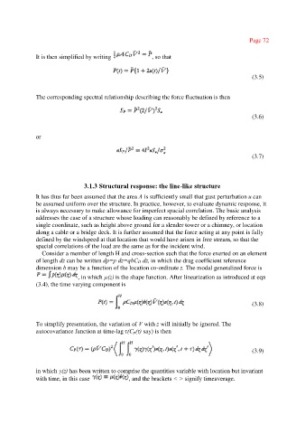
It is then simplified by writing , so that

(3.5)

The corresponding spectral relationship describing the force fluctuation is then

(3.6)

or

(3.7)

3.1.3 Structural response: the line-like structure

It has thus far been assumed that the area A is sufficiently small that gust perturbation u can
be assumed uniform over the structure. In practice, however, to evaluate dynamic response, it
is always necessary to make allowance for imperfect spacial correlation. The basic analysis
addresses the case of a structure whose loading can reasonably be defined by reference to a
single coordinate, such as height above ground for a slender tower or a chimney, or location
along a cable or a bridge deck. It is further assumed that the force acting at any point is fully
defined by the windspeed at that location that would have arisen in free stream, so that the
spacial correlations of the load are the same as for the incident wind.
Consider a member of length H and cross-section such that the force exerted on an element
of length dz can be written dp=p dz=qbCD dz, in which the drag coefficient reference
dimension b may be a function of the location co-ordinate z. The modal generalized force is
, in which µ(z) is the shape function. After linearization as introduced at eqn
(3.4), the time varying component is

(3.8)

To simplify presentation, the variation of V with z will initially be ignored. The
autocovariance function at time-lag τCp(τsay) is then
(
)

(3.9)

(
in which γz) has been written to comprise the quantities variable with location but invariant
with time, in this case , and the brackets < > signify timeaverage.