Page 55 - Dynamic Vision for Perception and Control of Motion

2.1 Three-dimensional (3-D) Space and Time 39

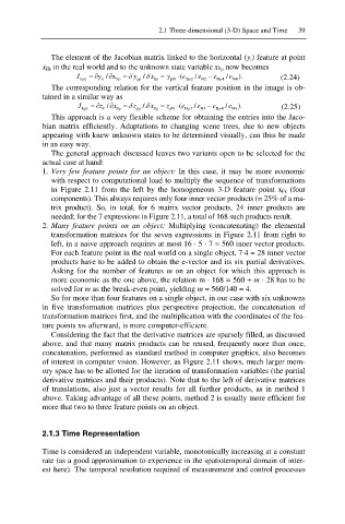
The element of the Jacobian matrix linked to the horizontal (y i) feature at point
x Fk in the real world and to the unknown state variable xS U now becomes
G
J kȡy w y/ x Sȡ G y pȡ / x y ˜ (e Dȡ2 / e e Dȡ4 e / N4 ). (2.24)
w
Sȡ
k
N2
pN
The corresponding relation for the vertical feature position in the image is ob-
tained in a similar way as
G
w
J w z / x G z / x z ˜ (e / e e / e ). (2.25)
kȡz k Sȡ pȡ Sȡ pN Dȡ3 N3 Dȡ4 N4
This approach is a very flexible scheme for obtaining the entries into the Jaco-
bian matrix efficiently. Adaptations to changing scene trees, due to new objects
appearing with knew unknown states to be determined visually, can thus be made
in an easy way.
The general approach discussed leaves two variants open to be selected for the
actual case at hand:
1. Very few feature points for an object: In this case, it may be more economic
with respect to computational load to multiply the sequence of transformations
in Figure 2.11 from the left by the homogeneous 3-D feature point x Fk (four
components). This always requires only four inner vector products (= 25% of a ma-
trix product). So, in total, for 6 matrix vector products, 24 inner products are
needed; for the 7 expressions in Figure 2.11, a total of 168 such products result.
2. Many feature points on an object: Multiplying (concatenating) the elemental
transformation matrices for the seven expressions in Figure 2.11 from right to
left, in a naive approach requires at most 16 · 5 · 7 = 560 inner vector products.
For each feature point in the real world on a single object, 7·4 = 28 inner vector
products have to be added to obtain the e-vector and its six partial derivatives.
Asking for the number of features m on an object for which this approach is
more economic as the one above, the relation m · 168 = 560 + m · 28 has to be
solved for m as the break-even point, yielding m = 560/140 = 4.
So for more than four features on a single object, in our case with six unknowns
in five transformation matrices plus perspective projection, the concatenation of
transformation matrices first, and the multiplication with the coordinates of the fea-
ture points xFk afterward, is more computer-efficient.
Considering the fact that the derivative matrices are sparsely filled, as discussed
above, and that many matrix products can be reused, frequently more than once,
concatenation, performed as standard method in computer graphics, also becomes
of interest in computer vision. However, as Figure 2.11 shows, much larger mem-
ory space has to be allotted for the iteration of transformation variables (the partial
derivative matrices and their products). Note that to the left of derivative matrices
of translations, also just a vector results for all further products, as in method 1
above. Taking advantage of all these points, method 2 is usually more efficient for
more that two to three feature points on an object.

2.1.3 Time Representation

Time is considered an independent variable, monotonically increasing at a constant
rate (as a good approximation to experience in the spatiotemporal domain of inter-
est here). The temporal resolution required of measurement and control processes