Page 54 - Dynamic Vision for Perception and Control of Motion

38 2 Basic Relations: Image Sequences – “the World”

with the last column of the old (intermediate) product matrix. This analytical in-
sight can save 75% of the computational steps for all matrices to the left if column
vectors are used and matrix multiplication starts from the right-hand side.
The derivative matrices for rotational variables have four nonzero elements.
These trigonometric functions have already been evaluated for the nominal case.
The nonzero elements appear in such a pattern that working with sets of row– or
column–vectors for matrices cuts in half the number of multiplications necessary
for the elements of the product matrix.
As a final step toward image coordinates, the leftmost matrix P for perspective
projection has to be applied. Note that this matrix product and the following scal-
ing operations with element e 4 (Equation 2.11) yield two feature positions y and z
in the image for each real-world feature. Thus, two Jacobian elements are also ob-
tained for each image feature.
To get from the partial derivative of the total homogeneous transformation ma-
trix T’ tU to the correspondingly varied feature position in the image, this matrix has
to be multiplied from the right-hand side by the 3-D feature vector xFk for the fea-
ture point (see Figure 2.11). This yields n vectors e DkU , U = 1 to n (6 in our case),
each of which has four components. This is shown in the lower part of Figure 2.11.
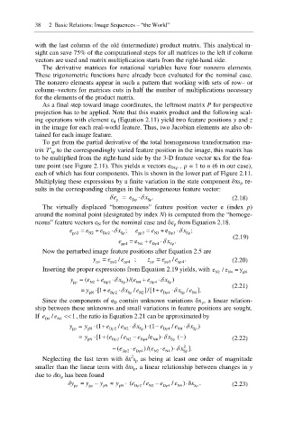
Multiplying these expressions by a finite variation in the state component GxS U re-
sults in the corresponding changes in the homogeneous feature vector:
e G e ˜ G x . (2.18)
ȡ Dȡ Sȡ
The virtually displaced “homogeneous” feature position vector e (index p)
around the nominal point (designated by index N) is computed from the “homoge-
neous” feature vectors e N for the nominal case and Ge U from Equation 2.18.
e e e ˜ G x ; e e e ˜ G x ;
pȡ2 N2 Dȡ2 Sȡ pȡ3 N3 Dȡ3 Sȡ
(2.19)
e pȡ4 e N4 e Dȡ4 ˜ G x Sȡ .
Now the perturbed image feature positions after Equation 2.5 are
y pȡ = e pȡ2 / e pȡ4 ; z pȡ = e pȡ3 /e pȡ4 . (2.20)
Inserting the proper expressions from Equation 2.19 yields, with e / e = y
N2 N4 pN
y = (e e ˜ G x ) /(e e ˜ G x )
pȡ N2 Dȡ2 Sȡ N4 Dȡ4 Sȡ
(2.21)
= y ˜ ˜ G x / e ]/[1 e ˜ G x / e ].

[1 e
pN Dȡ2 Sȡ N2 Dȡ4 Sȡ N4
Since the components of e D contain unknown variations Gx U, a linear relation-
ship between these unknowns and small variations in feature positions are sought.
If e / e 1, the ratio in Equation 2.21 can be approximated by
D4 N4

˜ G

y y ˜ (1 e / e ˜ x ) (1 e / e ˜ G x )
pȡ pN Dȡ2 N2 Sȡ Dȡ4 N4 Sȡ
y ˜ [1 (e / e e /e )˜ x ( )
G

pN Dȡ2 N2 Dȡ4 N4 Sȡ (2.22)

(e e ˜ ) /(e ˜ e )˜ G x 2 ].
Dȡ2 Dȡ4 N2 N4 Sȡ
2
Neglecting the last term with Gx S U as being at least one order of magnitude
smaller than the linear term with GxS U, a linear relationship between changes in y
due to GxS U has been found
˜
įy pȡ = y pȡ y pN | y pN ˜ (e Dȡ2 / e N2 e Dȡ4 / e N4 ) įx . (2.23)
Sȡ