Page 53 - Dynamic Vision for Perception and Control of Motion

2.1 Three-dimensional (3-D) Space and Time 37

2.1.2.2 Concatenations and Efficient Computation Schemes

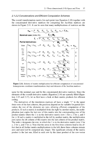
The overall transformation matrix for each point (see Equation 2.10) together with
the concatenated derivative matrices for computing the Jacobian matrices are
shown in Figure 2.11. It can be seen that many multiplications of matrices are the

e kN = P R Tc R \c T Rc T Ro R \c x Fk = T x Fk
t
Nominal case (index N): T =M 5
t
T t = P R Tc R \c T Rc T Ro R \c x Fk
Partial derivatives: M 4 V 1
State ˜ e / ˜ \ o = P R Tc R \c T Rc T Ro R’ \o x Fk = e DU
k
U = 1 .. 6
Per- V
tur- 1
ba- ˜ e / ˜ x co = P R Tc R \c T Rc T’ Rox R \c x Fk 2
k
tion
˜ e / ˜ y = P R R T T’ R x
k oR Tc \c Rc Roy \c Fk 3
eff -
ects V 2
˜ e / ˜ y = P R R T’ T R x 4
on k gc Tc \c Rc Ro \c Fk
V M 1
‘homo - 3
gene - ˜ e / ˜ \ c = P R Tc R’ \c T Rc T Ro R \c x Fk 5
k
ous’
V 4 M 2
feature
vector ˜ e / ˜ 4 c = P R’ Tc R \c T Rc T Ro R \c x Fk 6
k
M
3
Figure 2.11. Scheme of matrix multiplication for efficient computation of concatenated
homogeneous coordinate transformations (top) and elements of the Jacobian matrices
same for the nominal case and for the concatenated derivative matrices. Since the
elements of the overall derivative matrix (Equation 2.14) are sparsely filled (Equa-
tion 2.15 and 2.17), let us first have a look at their matrix products for efficient
coding.
The derivatives of the translation matrices all have a single “1” in the upper
three rows of the last columns, the positions depend on the variable for partial deri-
vation; the rest of the elements are zero, allowing efficient computation of the
products. If such a matrix is multiplied from the right by another matrix, the multi-
plication just copies the last row of this matrix into the corresponding row of the
product matrix where the 1 is in the derivative matrix (row 1 for x, 2 for y, and 3
for z). If such a matrix is multiplied to the left by another matrix, the multiplication
just copies the ith column of this matrix into the last column of the product matrix.
The index i designates the row, in which the 1 is in the derivative matrix (row 1 for
x, 2 for y, and 3 for z). Note that the zeros in the first three columns lead to the ef-
fect that in all further matrix multiplications to the left, these three columns remain
zero and need not be computed any longer. The significant column of the matrix
product is the last one, filled in each row by the inner product of the row-vector