Page 48 - Dynamic Vision for Perception and Control of Motion

32 2 Basic Relations: Image Sequences – “the World”

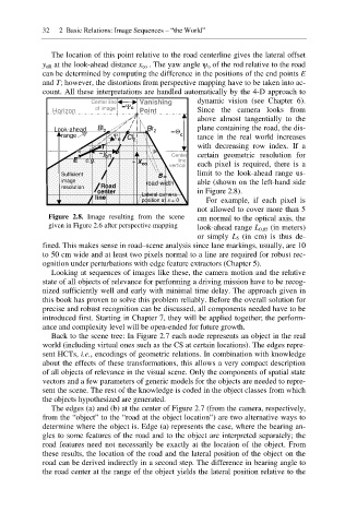
The location of this point relative to the road centerline gives the lateral offset
y oR at the look-ahead distance x co . The yaw angle \ o of the rod relative to the road
can be determined by computing the difference in the positions of the end points E
and T; however, the distortions from perspective mapping have to be taken into ac-
count. All these interpretations are handled automatically by the 4-D approach to
Center line Vanishing dynamic vision (see Chapter 6).
of image í<c
Horizon Point Since the camera looks from
o
above almost tangentially to the
Look-ahead Bl 2 o o o Br 2 í4 plane containing the road, the dis-
range < o Cl 2 c tance in the real world increases
o T with decreasing row index. If a
íy o
o oR Center certain geometric resolution for
E c.g. ~ x co vertical each pixel is required, there is a
line
Sufficient B= limit to the look-ahead range us-
image road width able (shown on the left-hand side
resolution Road
center in Figure 2.8).
line Lateral camera
position at x = 0 For example, if each pixel is
not allowed to cover more than 5
Figure 2.8. Image resulting from the scene cm normal to the optical axis, the
given in Figure 2.6 after perspective mapping look-ahead range L 0.05 (in meters)
or simply L 5 (in cm) is thus de-
fined. This makes sense in road–scene analysis since lane markings, usually, are 10
to 50 cm wide and at least two pixels normal to a line are required for robust rec-
ognition under perturbations with edge feature extractors (Chapter 5).
Looking at sequences of images like these, the camera motion and the relative
state of all objects of relevance for performing a driving mission have to be recog-
nized sufficiently well and early with minimal time delay. The approach given in
this book has proven to solve this problem reliably. Before the overall solution for
precise and robust recognition can be discussed, all components needed have to be
introduced first. Starting in Chapter 7, they will be applied together; the perform-
ance and complexity level will be open-ended for future growth.
Back to the scene tree: In Figure 2.7 each node represents an object in the real
world (including virtual ones such as the CS at certain locations). The edges repre-
sent HCTs, i.e., encodings of geometric relations. In combination with knowledge
about the effects of these transformations, this allows a very compact description
of all objects of relevance in the visual scene. Only the components of spatial state
vectors and a few parameters of generic models for the objects are needed to repre-
sent the scene. The rest of the knowledge is coded in the object classes from which
the objects hypothesized are generated.
The edges (a) and (b) at the center of Figure 2.7 (from the camera, respectively,
from the “object” to the “road at the object location”) are two alternative ways to
determine where the object is. Edge (a) represents the case, where the bearing an-
gles to some features of the road and to the object are interpreted separately; the
road features need not necessarily be exactly at the location of the object. From
these results, the location of the road and the lateral position of the object on the
road can be derived indirectly in a second step. The difference in bearing angle to
the road center at the range of the object yields the lateral position relative to the