Page 46 - Dynamic Vision for Perception and Control of Motion

30 2 Basic Relations: Image Sequences – “the World”

rows of the HTMs in Equation 2.8. It has not been done here because the direction
of the local road tangents would not be the same for a curved road. Therefore, be-
fore performing the second translation to the origin of the camera CS, a rotation
around the vertical axis by the difference F in local road direction would have to be
inserted (yielding another rotation matrix R Fco between T Rc and T Ro.
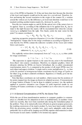
Now the two rotation-angles \ c and 4 c for the optical axis of the camera have to
be applied. Since \ c according to the definition has to be applied first, R \c has to
stand to the right because this matrix will be encountered first when the column-
vector x o is multiplied from the right. This finally yields the state vector for the
point T in camera coordinates:

x R \ c ˜ R T c T ˜ Rc T ˜ Ro ˜ R \ o ˜ x . (2.9)
co
o
Applying perspective projection (Equation (2.4) to this 3-D-point x co yields the
“homogeneous” feature data for the image coordinates e according to Equation 2.5;
note that the five HTMs contain the unknown variables of the vision task written
below each matrix:
e [ PR ˜ p ˜ T c R ˜ \ c T ˜ Rc T ˜ Ro R \ o ] x ˜ o T ˜ tot x .
o
(2.10)
unknowns: ș , ȥ , y (x ,y ) ȥ !
c c gc co oR o
T
The explicitly written down (transposed) form (e) = (e 1, e 2, e 3, e 4) then yields
the image coordinates
e
e
y i / ; e 2 e 4 z i / . (2.11)
3
4
The expression in square brackets is the same for any point to be transformed
from object- into camera- coordinates. Therefore, in computer graphics, where all
elements entering the HTMs are known beforehand, the so-called concatenated
transformation matrix T tot is computed as the product of all single HTMs once for
each object and aspect condition. A single matrix-vector multiplication T tot · x o then
yields the position in homogeneous feature coordinates for the image of a point on
the object at x o in object-centered coordinates. Equation 2.11 finally gives the im-
age coordinates.
Note that these coordinates are real numbers, which means that the positions of
the points mapped into the image are known to subpixel accuracy. If measurements
of image features (Chapter 5) can be done to subpixel accuracy, too, the methods
applied in recursive estimation (see Chapter 6) yield improved results by not
rounding off feature coordinates to integer numbers (as is often done in a naive ap-
proach).

2.1.1.6 General Concatenations of HCTs; the Scene Tree
While the use of these transformation matrices in computer graphics is common-
place as a flexible tool for adaptation to new or modified tasks, in machine vision,
until very recently, they have been exploited only during the formulation phase of
the problem. Then, to be numerically more efficient on general-purpose processors,
the resulting expressions of the matrix product T tot have been hand-coded, initially.
With the processing power available now, more easily adaptable codes become
preferable; this is achieved by keeping each HTMs separate until numerical evalua-
tion because in each matrix variables to be iterated may appear.