Page 47 - Dynamic Vision for Perception and Control of Motion

2.1 Three-dimensional (3-D) Space and Time 31

The challenge in machine vision as opposed to computer graphics is that some
of the transformation parameters entering the matrices are not known beforehand
but are the unknowns of the vision process, which have to be determined from im-
age sequence analysis. Therefore, in each transformation, its sensitivity to small
parameter changes has to be determined to compute the corresponding overall
“Jacobian” matrices (JM, the first-order approximation for the nonlinear functional
relationship describing the mapping of features on objects in the real world to those
measured in the images). This rather compute-intensive operation and an efficient
implementation will be discussed in Section 2.1.2.
The tendency toward separation of application-oriented aspects from those
geared to the general methods of dynamic vision required a major change from the
initial approach with respect to handling homogeneous coordinates. Concatenation
is shifted to the evaluation of the scene model at runtime; then, both the nominal
total HTM and the partial-derivative matrices for all unknown parameters and state
variables are computed in conjunction (maybe numerically). This allows efficient
use of intermediate results and makes the setup of new problems much easier for
the user. The corresponding representation scheme for all objects and CSs in a so-
called “scene tree” has been developed by D. Dickmanns (1997) and will be dis-
cussed in the following paragraphs.
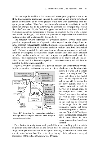
Figure 2.7 without the shaded areas gives an example of a scene tree for describ-
ing the geometrical relations among several objects of relevance for the vision task
shown in Figure 2.6 a single
[3 (known) translations], Vehicle body camera on a straight road. The
2 rotations \ , 4 cb nodes and edges in the shaded
cb
3 translations,
Camera 3 rotations areas on the right-hand side
(general case)
1 translation y gc , and on top will be needed for
2 rotations \ , 4 the more general case of a
c c road nearby
range & camera onboard a vehicle
Perspective bearing Curvature
projection (a) parameters moving on a curved road. In
Chip C N0 , C N1 (L N ) the straight road scene, the
object
Frame grabber Road at ob- “object” represents the rod on
Pixel (b) ject location the road at some look-ahead
position
1 translation y go Curvature distance x co; its lateral position
1 rotation \ o parameters
C F0 , C F1 (L F ) on the road can be recovered
Image in
storage in the image from the road
location ‘Vanishing Road boundaries nearby and from
point’ far away
for straight road
the vanishing point at the hori-
zon (see Figure 2.8).The figure
Figure 2.7. Scene tree for representing spatial rela-
shows the resulting image, into
tionships between objects seen and their image in
which some labels for later
perspective projection
image interpretation have been
inserted.
For a horizontal straight road with parallel lines, the vanishing point, at which
all parallel lines intersect, lies on the horizon line. Its distance components to the
image center yield the direction of the optical axis: í\ c to the direction of the road
and íT c to the horizon line. The center of gravity (cg) of the rod has the averaged
coordinates of the end points E and T in 3-D space.