Page 91 - Dynamics and Control of Nuclear Reactors

84 CHAPTER 7 Reactivity feedbacks

FIG. 7.7
Block diagram representation of destabilizing negative feedback example. Note that when
gain K is less than zero, the feedback becomes negative.

Fig. 7.7 shows the block diagram representation of the system defined by the
above equations with K ¼ 5.
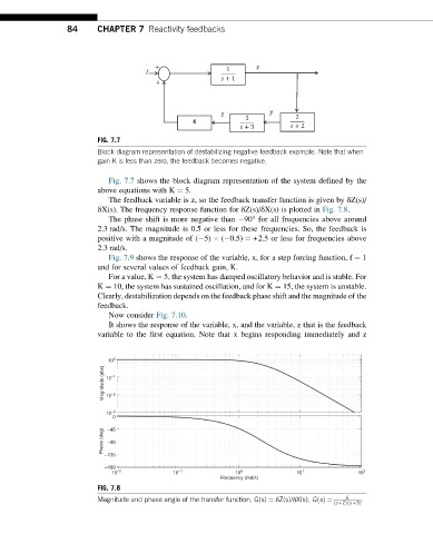
The feedback variable is z, so the feedback transfer function is given by δZ(s)/
δX(s). The frequency response function for δZ(s)/δX(s) is plotted in Fig. 7.8.
The phase shift is more negative than 90° for all frequencies above around
2.3 rad/s. The magnitude is 0.5 or less for these frequencies. So, the feedback is
positive with a magnitude of ( 5) ( 0.5) ¼ +2.5 or less for frequencies above
2.3 rad/s.
Fig. 7.9 shows the response of the variable, x, for a step forcing function, f ¼ 1
and for several values of feedback gain, K.
For a value, K ¼ 5, the system has damped oscillatory behavior and is stable. For
K ¼ 10, the system has sustained oscillation, and for K ¼ 15, the system is unstable.
Clearly, destabilization depends on the feedback phase shift and the magnitude of the
feedback.
Now consider Fig. 7.10.
It shows the response of the variable, x, and the variable, z that is the feedback
variable to the first equation. Note that x begins responding immediately and z

10 0
Magnitude (abs) 10 –1

–2
10
10 –3
0
Phase (deg) –45
–90
–135
–180
10 –2 10 –1 10 0 10 1 10 2
Frequency (rad/s)
FIG. 7.8
6
Magnitude and phase angle of the transfer function, G(s) ¼ δZ(s)/δX(s), GsðÞ ¼ .
ð
ð s +2Þ s +3Þ