Page 119 - Dynamics of Mechanical Systems

0593_C04*_fm Page 100 Monday, May 6, 2002 2:06 PM

100 Dynamics of Mechanical Systems

1 rev/sec
n
z
n
x L R
n 30° 30°
y
O W
FIGURE 4.9.3
Sports car steering wheel W and 6 in
left and right hands L and R.

or

S L
V = 22 381 n − 1 571 n + 2 721 n ft sec (4.9.17)
.
.
.
x y z
and
S L n ) y ( z)
a =−19 36. n + − ( 5 529. × 0 433. n + 0 25. n
y y
[ ( z)]
+(6 283. n − 0 88. n z) × (6 283. n − 0 88. n z) × 0 433. n + 0 25. n (4.9.18)
x x y
=−2 765 n − 36 79. n − 9 87. n ft sec 2
.
x y z
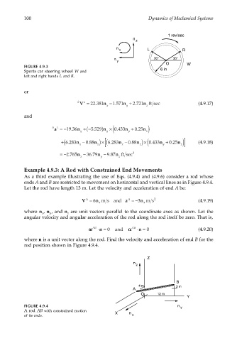
Example 4.9.3: A Rod with Constrained End Movements
As a third example illustrating the use of Eqs. (4.9.4) and (4.9.6) consider a rod whose
ends A and B are restricted to movement on horizontal and vertical lines as in Figure 4.9.4.
Let the rod have length 13 m. Let the velocity and acceleration of end A be:

A
A
V = 6 n m s and a = −3 n m s 2 (4.9.19)
x
x
where n , n , and n are unit vectors parallel to the coordinate axes as shown. Let the
z
y
x
angular velocity and angular acceleration of the rod along the rod itself be zero. That is,
ωω AB ⋅n = 0 and αα AB ⋅n = 0 (4.9.20)
where n is a unit vector along the rod. Find the velocity and acceleration of end B for the
rod position shown in Figure 4.9.4.

Z
n
z

B
4 m 3 m
A
O 12 m
Y
FIGURE 4.9.4 n y
A rod AB with constrained motion X n
of its ends. x