Page 306 - Dynamics of Mechanical Systems

0593_C09_fm Page 287 Monday, May 6, 2002 2:50 PM

Principles of Impulse and Momentum 287

Finally, by integrating in Eq. (9.5.7) we have:

t 2 t 2 t 2
I = ∫ Fdt = ∫ M a dt = ∫ M v (d G dt )dt
G
(9.5.8)
t 1 t 1 t 1
= M v () − M v () = L() − ()
L t
t
t
t
G 2 G 1 2 1
or
I =∆ L (9.5.9)

where L represents the linear momentum of S as in Eq. (9.3.2).
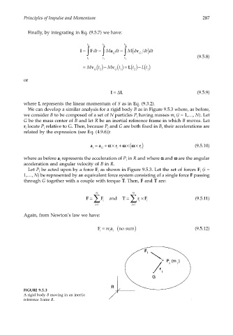
We can develop a similar analysis for a rigid body B as in Figure 9.5.3 where, as before,
we consider B to be composed of a set of N particles P having masses m (i = 1,…, N). Let
i
i
G be the mass center of B and let R be an inertial reference frame in which B moves. Let
r locate P relative to G. Then, because P and G are both fixed in B, their accelerations are
i
i
i
related by the expression (see Eq. (4.9.6)):
a = a + αα × r + ωω ×(ωω × r ) (9.5.10)
i G i i
where as before a represents the acceleration of P in R and where αα αα and ωω ωω are the angular
i
i
acceleration and angular velocity of B in R.
Let P be acted upon by a force F as shown in Figure 9.5.3. Let the set of forces F (i =
i
i
i
1,…, N) be represented by an equivalent force system consisting of a single force F passing
through G together with a couple with torque T. Then, F and T are:
N N
F = F and T = r × F (9.5.11)
∑ i ∑ i i
= i 1 = i 1

Again, from Newton’s law we have:

F = m a ( no sum ) (9.5.12)
i i i

FIGURE 9.5.3
A rigid body B moving in an inertia
reference frame R.