Page 307 - Dynamics of Mechanical Systems

0593_C09_fm Page 288 Monday, May 6, 2002 2:50 PM

288 Dynamics of Mechanical Systems

By substituting from Eqs. (9.5.10) and (9.5.12) into Eq. (9.5.11) we have:

F = M a (9.5.13)
G

where M is the mass of B.
Finally, by integrating in Eq. (9.5.13) we obtain (as in Eqs. (9.5.8) and (9.5.9)):

I =∆ L (9.5.14)

where now L represents the linear momentum of B.
Observe the identical formats of Eqs. (9.5.3), (9.5.9), and (9.5.14) for a single particle, a
set of particles, and a rigid body.

9.6 Principle of Angular Impulse and Momentum
We can develop expressions analogous to Eqs. (9.5.3), (9.5.9), and (9.5.14) for angular
impulse and angular momentum. The development here, however, has the added feature
of involving a reference point (or object point). Because angular momentum is always
computed relative to a point, the choice of that point may affect the form of the relation
between angular impulse and angular momentum.
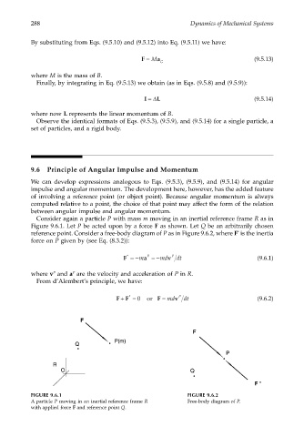
Consider again a particle P with mass m moving in an inertial reference frame R as in
Figure 9.6.1. Let P be acted upon by a force F as shown. Let Q be an arbitrarily chosen
reference point. Consider a free-body diagram of P as in Figure 9.6.2, where F is the inertia
*
force on P given by (see Eq. (8.3.2)):

*
P
P
F =−m a =−md v dt (9.6.1)
where v and a are the velocity and acceleration of P in R.
P
P
From d’Alembert’s principle, we have:
+
*
P
FF = or F = md v dt (9.6.2)
0

FIGURE 9.6.1 FIGURE 9.6.2
A particle P moving in an inertial reference frame R Free-body diagram of P.
with applied force F and reference point Q.