
Page 466 - Dynamics of Mechanical Systems
P. 466
0593_C13_fm Page 447 Monday, May 6, 2002 3:21 PM
Introduction to Vibrations 447
where F and p are constants. The governing equation then becomes:
0
+
mx kx = Acos pt (13.4.3)
˙˙
From Eqs. (13.2.32) through (13.2.35) we see that the general solution of Eq. (13.4.3) is:
F (
+
x = Acosω t Bsinω t + [ 0 k mp )] cos pt (13.4.4)
−
2
where as before A and B are constants to be determined from auxiliary conditions (such
as initial conditions) and where ω is defined as:
D
ω = km (13.4.5)
2
Consider the last term, [F /(k – mp )]cospt of Eq. (13.4.4). Observe that if p has values
2
0
nearly equal to k/m (that is, if p is nearly equal to ω) the denominator becomes very small,
producing large-amplitude oscillation. Indeed, if p is equal to ω, the oscillation amplitude
becomes unbounded. This means that by stimulating the mass B with a periodic force
having a frequency nearly equal to ω (that is, km ), the amplitude of the resulting oscillation
becomes unbounded.
The quantity km is called the natural frequency of the system. When the frequency of
the loading function is equal to the natural frequency, giving rise to a large-amplitude
response, we have the phenomenon commonly referred to as resonance.
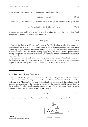
13.5 Damped Linear Oscillator
Consider next the damped linear oscillator as depicted in Figure 13.5.1. This is the same
system we considered in the previous sections, but here the movement of the mass B is
restricted by a “damper” in the form of a dashpot. For simplicity of illustration, we will
assume viscous damping, where the force exerted by the dashpot on B is proportional to
the speed of B and directed opposite to the motion of B with c being the constant of
proportionality. That is, the damping force F on B is:
D
F =− ˙ n (13.5.1)
cx
D
where n is a unit vector in the positive X direction as shown in Figure 13.5.1.
c
B
k
m
n
FIGURE 13.5.1 x
A damped mass–spring system.