Page 470 - Dynamics of Mechanical Systems

0593_C13_fm Page 451 Monday, May 6, 2002 3:21 PM

Introduction to Vibrations 451

j

i n 2
O
P
1

P
2 n
x x 1
1 2
P
3
T
n
3
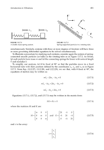
FIGURE 13.7.1 FIGURE 13.7.2
A double mass–spring system. Spring-supported particles in a rotating tube.
simultaneously. Similarly, systems with three or more degrees of freedom will have three
or more governing differential equations to be solved simultaneously.
To illustrate a procedure for studying such systems, consider again the system of spring-
connected smooth particles (or balls) in the rotating tube as in Figure 13.7.2. As before,
let each particle have mass m and let the connecting springs be linear with natural length
and modulus k.
To simplify our analysis, let θ be fixed at 90° so that the particles move in a fixed
horizontal tube with their position defined by the coordinates x , x , and x as in Figure
1
3
2
13.7.3. From Eqs. (12.2.27), (12.2.28), and (12.2.29), we see that, with θ fixed at 90°, the
equations of motion may be written as:
mx ˙˙ + 2 kx − kx = 0 (13.7.1)
1 1 2

mx ˙˙ − kx + 2 kx − kx = 0 (13.7.2)
2 1 2 3
mx ˙˙ − kx + 2 kx = 0 (13.7.3)
3 2 3

Equations (13.7.1), (13.7.2), and (13.7.3) may be written in the matrix form:

+
˙˙
Mx Kx = 0 (13.7.4)
where the matrices M and K are:

 m 0 0  2 k − k 0 
   
M = 0 m 0 and K = − k k 2 − k  (13.7.5)



  0 0 m    0 − k 2 k  
and x is the array:

x  
1
 
x =   (13.7.6)
x
2
x  
 
3