
Page 467 - Dynamics of Mechanical Systems
P. 467
0593_C13_fm Page 448 Monday, May 6, 2002 3:21 PM
448 Dynamics of Mechanical Systems
x
t
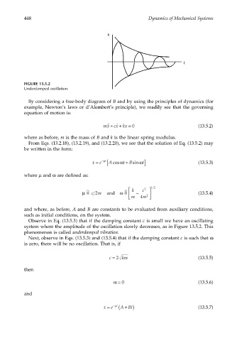
FIGURE 13.5.2
Underdamped oscillation.
By considering a free-body diagram of B and by using the principles of dynamics (for
example, Newton’s laws or d’Alembert’s principle), we readily see that the governing
equation of motion is:
+
+
˙˙
˙
mx cx kx = 0 (13.5.2)
where as before, m is the mass of B and k is the linear spring modulus.
From Eqs. (13.2.18), (13.2.19), and (13.2.20), we see that the solution of Eq. (13.5.2) may
be written in the form:
−µ
x = e [ cos ω t Bsin ω t] (13.5.3)
+
t
A
where µ and ω are defined as:
/
D D k c 2 12
µ = cm and ω = − (13.5.4)
2
m 4 m 2
and where, as before, A and B are constants to be evaluated from auxiliary conditions,
such as initial conditions, on the system.
Observe in Eq. (13.5.3) that if the damping constant c is small we have an oscillating
system where the amplitude of the oscillation slowly decreases, as in Figure 13.5.2. This
phenomenon is called underdamped vibration.
Next, observe in Eqs. (13.5.3) and (13.5.4) that if the damping constant c is such that ω
is zero, there will be no oscillation. That is, if
c = 2 km (13.5.5)
then
ω= 0 (13.5.6)
and
−µ
x = e ( A Bt) (13.5.7)
+
t