Page 463 - Dynamics of Mechanical Systems

0593_C13_fm Page 444 Monday, May 6, 2002 3:21 PM

444 Dynamics of Mechanical Systems

B
k
m frictionless

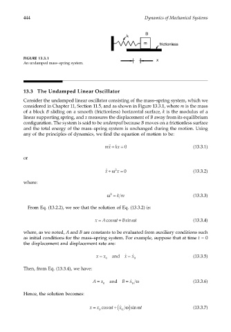
FIGURE 13.3.1 x
An undamped mass–spring system.

13.3 The Undamped Linear Oscillator
Consider the undamped linear oscillator consisting of the mass–spring system, which we
considered in Chapter 11, Section 11.5, and as shown in Figure 13.3.1, where m is the mass
of a block B sliding on a smooth (frictionless) horizontal surface, k is the modulus of a
linear supporting spring, and x measures the displacement of B away from its equilibrium
configuration. The system is said to be undamped because B moves on a frictionless surface
and the total energy of the mass–spring system is unchanged during the motion. Using
any of the principles of dynamics, we find the equation of motion to be:

+
˙˙
mx kx = 0 (13.3.1)
or

˙˙ x + ω 2 x = 0 (13.3.2)

where:

2
ω = km (13.3.3)
From Eq. (13.2.2), we see that the solution of Eq. (13.3.2) is:

x = Acosω t Bsinω t (13.3.4)
+

where, as we noted, A and B are constants to be evaluated from auxiliary conditions such
as initial conditions for the mass–spring system. For example, suppose that at time t = 0
the displacement and displacement rate are:

x = x and ˙ x = ˙ (13.3.5)
x
0 0
Then, from Eq. (13.3.4), we have:

A = x and B = ˙ ω (13.3.6)
x
0 0
Hence, the solution becomes:

x = x cosω x ˙ ω )sinω t (13.3.7)
0 t +( 0