Page 459 - Dynamics of Mechanical Systems

0593_C13_fm Page 440 Monday, May 6, 2002 3:21 PM

440 Dynamics of Mechanical Systems

where A and B are constants that may be evaluated by auxiliary conditions (initial condi-
tions or boundary conditions). (We can verify that the expression of Eq. (13.2.2) is indeed a
solution of Eq. (13.2.1) by direct substitution. It is in fact a general solution, as cosωt and
sinωt are independent functions and there are two arbitrary constants, A and B.)
Through use of trigonometric identities, we can express Eq. (13.2.2) in the form:

ˆ
x = Acos (ω t + ) φ (13.2.3)

where  and φ are constants. To develop this, recall the identity:

(
α
+
cos αβ) ≡ cos cosβ − sin sinβ (13.2.4)
α
Then, by thus expanding the expression of Eq. (13.2.3) we have:
ˆ
ˆ
ˆ
+
ω
ω
A cos ω ( t φ) = A cos t cosφ − A sin t sinφ (13.2.5)
By comparing this with Eq. (13.2.2), we have:
ˆ
ˆ
A = Acosφ B = Asinφ
(13.2.6)
A = A + B 2 tanφ = − B A
2
ˆ 2
In the expression  cos(ωt + φ) of Eq. (13.2.3),  is the amplitude, ω is the circular frequency,
and φ is the phase.
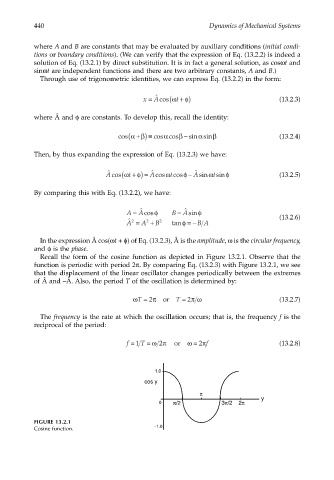
Recall the form of the cosine function as depicted in Figure 13.2.1. Observe that the
function is periodic with period 2π. By comparing Eq. (13.2.3) with Figure 13.2.1, we see
that the displacement of the linear oscillator changes periodically between the extremes
of  and –Â. Also, the period T of the oscillation is determined by:

ωT = 2 π or T = 2 π ω (13.2.7)

The frequency is the rate at which the oscillation occurs; that is, the frequency f is the
reciprocal of the period:

ω
2
f = 1 T = ωπ or = 2π f (13.2.8)

1.0
cos y
π
y
0 π/2 3π/2 2π

FIGURE 13.2.1
- 1.0
Cosine function.