Page 158 - Earth's Climate Past and Future

134 PART III • Orbital-Scale Climate Change

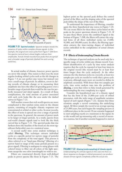
Higher highest point on the spectral peak defines the central
100,000 23,000 period of the filter, and the sloping sides of the spectral
41,000
peak define the shape of the rest of the filter.
To understand the importance of filtering, consider
Line spectra again the three hypothetical sine waves in Figure 7-20.
Power (sine waves)
We can create filters for these three cycles based on the
peaks in the power spectrum shown in Figure 7-21. If
Typical
real-world we pass these filters across the combined signal at the
Lower spectra bottom of Figure 7-20B, the filters will extract the orig-
100 50 25 20 15 10 inal form of all three individual cycles (at 23,000,
Period (thousands of years) 41,000, and 100,000 years). In effect, the filtering oper-
ation extracts the time-varying shapes of individual
FIGURE 7-21 Spectral analysis Spectral analysis reveals the cycles embedded in the complexities of actual climate
presence of cycles within complex climate signals. In this records.
example, the original sine wave cycles from Figure 7–20A form
line spectra (vertical bars) whose heights indicate their 7-9 Effects of Undersampling Climate Records
amplitudes. Actual climate records have peaks that are spread
over a broader range of periods (dashed line and curving The technique of spectral analysis can be used only for a
solid line). specific range of cycles within any climate record. Con-
fident identification of a cycle by time series analysis
requires that the cycle be repeated at least four times in
the original record (the record must be at least four
In actual studies of climate, however, power spectra times longer than the cycle analyzed). At the other
are never this simple. One reason is that even the most extreme (for the shortest cycles in a record), at least two
regular-looking orbital cycles such as the tilt changes in samples per cycle are needed to verify that a given cycle
Figure 7-4 are not perfect sine waves but instead vary is present, although many more are needed to define its
over a small range of periods. In addition, errors in dat- amplitude accurately. With fewer than two samples per
ing records of climate change or in measuring their cycle, time series analysis runs into the problem of
amplitude also have the effect of spreading power over a aliasing, a term that refers to false trends generated by
broader range of periods than would be the case for per- undersampling the true complexity in a signal.
fectly measured and dated signals. As a result of these Consider the hypothetical case of a climatic signal
complications, the total amount of power associated that has the form of the 23,000-year cycle of orbital
with each cycle looks like the area under the dashed precession, with the wide range of amplitude variation
curves in Figure 7-21. typical of such signals (Figure 7-22). Assume that three
Still another reason that real-world spectra are more scientists sample a record containing this underlying
complicated is that random noise exists in the climate signal. All three sample the record at an average spacing
system, consisting of irregular climatic responses not of 23,000 years, but each begins the sampling process at
concentrated at orbital or other cycles. In most records, a different place in the record. If one scientist happened
the effect of noise is spread out over a range of periods to start sampling exactly at a maximum in the signal, he
in the spectrum. In general, the amount of power tends or she would end up measuring only a record of succes-
to be larger at longer periods. As a result, spectra from sive maxima, but if another scientist happened to start at
real-world climatic signals tend to look like the thick
curved line in Figure 7-21. The spectral peaks that rise
farthest above the baseline of the trend are the most sig- Incorrect signals Actual signal
nificant (believable) ones in a statistical sense. caused by undersampling
A second useful time series analysis technique is
called filtering. This technique extracts individual
cycles at a specific period (or narrow range of periods) Amplitude of climate signal
from the complexity of the total signal. This process is
often referred to as “band-pass filtering” (filtering of a
narrow band or range of the many periods present in a
given signal). Filtering is analogous to using glasses with Time
colored lenses to filter out all colors of the light spec- FIGURE 7-22 Aliasing (undersampling) of climate signals
trum except the one color (wavelength) we wish to see. Undersampling of a climate signal (in this case one that is a
Filters are constructed directly from well-defined direct response to changes in orbital precession) can produce
peaks in power spectra like those in Figure 7-21. The aliased climate signals completely unlike the actual one.