Page 63 - Electric Drives and Electromechanical Systems

56 Electric Drives and Electromechanical Systems

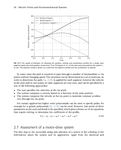
FIG. 2.11 The results of Example 2.4, showing the position, velocity and acceleration profiles for a single cubic
segment where the joint position moves from 15 to 75 degrees in 3 s, at the start and end positions the system is
at rest. The distance moved is shown as a solid line, the speed as dotted and the acceleration as dashed.

In many cases the path is required to pass through a number of intermediate or via
points without changing speed. The via points can be determined as a set of positions. In
order to determine the path, Eq. (2.36) is applied for each segment, however the velocity
at the start and/or end points of cubic segments are non-zero, and can be specified by a
one of the following approaches:

The user specifies the velocities at the via point.
The system computes a velocity based on a function of the joint position.
The system computes the velocity at the via point to maintain constant accelera-
tion through the via point.

For certain applications higher order polynomials can be used to specify paths, for
example for a quintic polynomial, Eq. (2.39) can be used. However, this needs all three
parameters at the start and finish to be specified, which gives a linear set of six equations
that require solving, to determine the coefficients of the profile,
2
3
4
qðtÞ¼ a 0 þ a 1 t þ a 2 t þ a 3 t þ a 4 t þ a 5 t 5 (2.39)

2.7 Assessment of a motor-drive system

The first step to the successful sizing and selection of a system is the collating of the
information about the system and its application. Apart from the electrical and