Page 144 - Electrical Properties of Materials

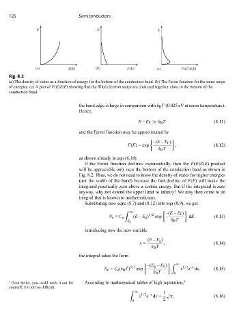
126 Semiconductors

E E E

(a) Z(E) (b) F(E) (c) F(E) Z(E)
Fig. 8.2
(a) The density of states as a function of energy for the bottom of the conduction band. (b) The Fermi function for the same range
of energies. (c) A plot of F(E)Z(E) showing that the filled electron states are clustered together close to the bottom of the
conduction band.

the band edge is large in comparison with k B T (0.025 eV at room temperature).
Hence,

E – E F k B T (8.11)
and the Fermi function may be approximated by

–(E – E F )
F(E)=exp , (8.12)
k B T
as shown already in eqn (6.18).
If the Fermi function declines exponentially, then the F(E)Z(E) product
will be appreciable only near the bottom of the conduction band as shown in
Fig. 8.2. Thus, we do not need to know the density of states for higher energies
(nor the width of the band) because the fast decline of F(E) will make the
integrand practically zero above a certain energy. But if the integrand is zero
anyway, why not extend the upper limit to infinity? We may then come to an
integral that is known to mathematicians.
Substituting now eqns (8.7) and (8.12) into eqn (8.9), we get

∞ –(E – E F )

N e = C e (E – E g ) 1/2 exp dE. (8.13)
k B T
E g
Introducing now the new variable
(E – E g )
x = , (8.14)
k B T
the integral takes the form

–(E g – E F )
∞
N e = C e (k B T) 3/2 exp x 1/2 –x (8.15)
e dx.
k B T 0
∗ Even better, you could work it out for According to mathematical tables of high reputation, ∗
yourself; it’s not too difficult.

∞ 1√
x 1/2 –x π, (8.16)
e dx =
0 2