Page 281 - Electrical Properties of Materials

Microscopic theory (phenomenological) 263

We can now rewrite eqn (11.19), for the case H =0, in the form,
T
b = L(b). (11.22)
3θ
M
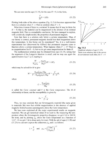
Plotting both sides of the above equation (Fig. 11.3) it becomes apparent that N m μ m
T θ T = θ T θ
there is a solution when T <θ but no solution when T >θ.
What does it mean if there is a solution? It means that M maybefinitefor
H = 0; that is, the material can be magnetized in the absence of an external
magnetic field. This is a remarkable conclusion. We have managed to explain,
with a relatively simple model, the properties of permanent magnets.
Note that there is a solution only below a certain temperature. Thus, if
our theory is correct, permanent magnets should lose their magnetism above
this temperature. Is this borne out by experiment? Yes, it is a well-known
experimental fact (discovered by Gilbert) that permanent magnets cease to 0 2 4 6 b
function above a certain temperature. What happens when T >θ?Thereis
Fig. 11.3
no magnetization for H = 0, but we do get some magnetization for finite H. Graphical solution of eqn (11.22).
The mathematical solution may be obtained from eqn (11.19), noting that There is no solution, that is the curves
the argument of the Langevin function is small, and we may use again the do not intersect each other, for T >θ.
~
approximation L(a) = a/3, leading to
M μ m μ 0
= (H + λM), (11.23)
N m μ m 3k B T
which may be solved for M to give
2
N m μ μ 0 /3k B C
m
M = 2 H = H, (11.24)
T – N m μ μ 0 λ/3k B T – θ
m
where
2
N m μ μ 0
m
C = (11.25)
3k B
is called the Curie constant and θ is the Curie temperature.The M–H
relationship is linear, and the susceptibility is given by
C
χ m = . (11.26)
T – θ
Thus, we may conclude that our ferromagnetic material (the name given
to materials like iron that exhibit magnetization in the absence of applied
magnetic fields) becomes paramagnetic above the Curie temperature.
We have now explained all the major experimental results on magnetic
materials. We can get numerical values if we want to. By measuring the tem-
perature where the ferromagnetic properties disappear, we get θ (it is 1043 K
for iron), and by plotting χ m above the Curie temperature as a function of
1/(T – θ) we get C (it is about unity for iron). With the aid of eqns (11.20) and
(11.25) we can now express the unknowns μ m and λ as follows:

1/2
θ 3 k B C
λ = and μ m = . (11.27)
C N m μ 0