Page 280 - Electrical Properties of Materials

262 Magnetic materials

At normal temperatures and reasonable magnetic fields, a 1 and
eqn (11.14) may be expanded to give
2
N m μ μ 0 H
m
M = , (11.15)
3k B T
leading to

2
Here χ m is definitely positive and N m μ μ 0
m
varies inversely with temperature. χ m = 3k B T . (11.16)
At the other extreme of very low temperatures all the magnetic dipoles line
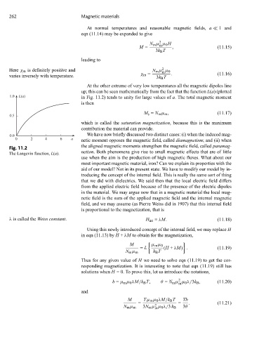
up; this can be seen mathematically from the fact that the function L(a) (plotted
1.0 L(a) in Fig. 11.2) tends to unity for large values of a. The total magnetic moment
is then

M s = N m μ m , (11.17)
0.5
which is called the saturation magnetization, because this is the maximum
contribution the material can provide.
0.0 We have now briefly discussed two distinct cases: (i) when the induced mag-
0 2 4 6 a
netic moment opposes the magnetic field, called diamagnetism; and (ii) when
the aligned magnetic moments strengthen the magnetic field, called paramag-
Fig. 11.2
netism. Both phenomena give rise to small magnetic effects that are of little
The Langevin function, L(a).
use when the aim is the production of high magnetic fluxes. What about our
most important magnetic material, iron? Can we explain its properties with the
aid of our model? Not in its present state. We have to modify our model by in-
troducing the concept of the internal field. This is really the same sort of thing
that we did with dielectrics. We said then that the local electric field differs
from the applied electric field because of the presence of the electric dipoles
in the material. We may argue now that in a magnetic material the local mag-
netic field is the sum of the applied magnetic field and the internal magnetic
field, and we may assume (as Pierre Weiss did in 1907) that this internal field
is proportional to the magnetization, that is
λ is called the Weiss constant. H int = λM. (11.18)

Using this newly introduced concept of the internal field, we may replace H
in eqn (11.13) by H + λM to obtain for the magnetization,

M μ m μ 0
= L (H + λM) . (11.19)
N m μ m k B T
Thus for any given value of H we need to solve eqn (11.19) to get the cor-
responding magnetization. It is interesting to note that eqn (11.19) still has
solutions when H = 0. To prove this, let us introduce the notations,
2
b = μ m μ 0 λM/k B T, θ = N m μ μ 0 λ/3k B , (11.20)
m
and
M Tμ m μ 0 λM/k B T Tb
= = . (11.21)
2
N m μ m 3N m μ μ 0 λ/3 k B 3θ
m