Page 234 - Electromagnetics

3.0
2.5
2.0
1.5 W
1.0
− ε
0.5
0.0
-0.5
−
-1.0 ε ε 0
-1.5
-2.0
Region of anomalous
-2.5
dispersion
0.0 0.5 1.0 1.5 2.0 2.5
ω/ω 0

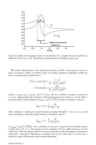
Figure 4.4: Real and imaginary parts of permittivity for a single resonance model of a
2
dielectric with /ω 0 = 0.2. Permittivity normalized by dividing by 0 (ω p /ω 0 ) .

The major characteristic of the dispersion relation (4.104) is the presence of one or
more resonances. Figure 4.4 shows a plot of a single resonance component, where we
have normalized the permittivity as
1 − ¯ω 2
2 ,
p 2
(˜ (ω) − 0 )/( 0 ¯ω ) =
2 ¯ 2
1 − ¯ω 2 + 4 ¯ω
2 ¯ω ¯
2 ,
p 2
2 ¯ 2
−˜ (ω)/( 0 ¯ω ) =
1 − ¯ω 2 + 4 ¯ω
¯
with ¯ω = ω/ω 0 , ¯ω p = ω p /ω 0 , and = /ω 0 . We see a distinct resonance centered at
ω = ω 0 . Approaching this resonance through frequencies less than ω 0 , we see that ˜
√
increases slowly until peaking at ωmax = ω 0 1 − 2 /ω 0 where it attains a value of
1 ¯ ω 2 p

˜ max = 0 + 0 .
¯
¯
4 (1 − )
After peaking, ˜ undergoes a rapid decrease, passing through ˜ = 0 at ω = ω 0 , and

then continuing to decrease until reaching a minimum value of
1 ¯ ω 2 p
˜ = 0 − 0
min 4 (1 + )
¯
¯
√

at ω min = ω 0 1 + 2 /ω 0 .As ω continues to increase, ˜ again increases slowly toward

a final value of ˜ = 0 . The regions of slow variation of ˜ are called regions of normal

dispersion, while the region where ˜ decreases abruptly is called the region of anomalous
dispersion. Anomalous dispersion is unusual only in the sense that it occurs over a
narrower range of frequencies than normal dispersion.
© 2001 by CRC Press LLC