Page 237 - Electromagnetics

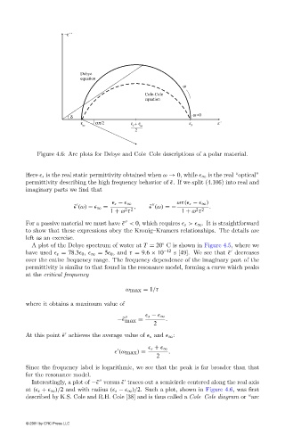
Figure 4.6: Arc plots for Debye and Cole–Cole descriptions ofa polar material.

Here s is the real static permittivity obtained when ω → 0, while ∞ is the real “optical”
permittivity describing the high frequency behavior of ˜ . If we split (4.106) into real and
imaginary parts we find that

ωτ( s − ∞ )
s − ∞

˜ (ω) − ∞ = , ˜ (ω) =− .
2 2
2 2
1 + ω τ 1 + ω τ
For a passive material we must have ˜ < 0, which requires s > ∞ . It is straightforward

to show that these expressions obey the Kronig–Kramers relationships. The details are
left as an exercise.
A plot of the Debye spectrum of water at T = 20 C is shown in Figure 4.5, where we
◦

have used s = 78.3 0 , ∞ = 5 0 , and τ = 9.6 × 10 −12 s [49]. We see that ˜ decreases
over the entire frequency range. The frequency dependence of the imaginary part of the
permittivity is similar to that found in the resonance model, forming a curve which peaks
at the critical frequency
ωmax = 1/τ
where it obtains a maximum value of

s − ∞
−˜ max = .

2
At this point ˜ achieves the average value of s and ∞ :

s + ∞

(ωmax ) = .
2
Since the frequency label is logarithmic, we see that the peak is far broader than that
for the resonance model.

Interestingly, a plot of −˜ versus ˜ traces outa semicircle centered along the real axis

at ( s + ∞ )/2 and with radius ( s − ∞ )/2. Such a plot, shown in Figure 4.6, was first
described by K.S. Cole and R.H. Cole [38] and is thus called a Cole–Cole diagram or “arc

© 2001 by CRC Press LLC