Page 238 - Electromagnetics

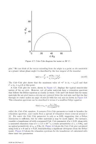
60

/ε 0
40
-ε

20

0
0 20 40 60
ε /ε 0

◦
Figure 4.7: Cole–Cole diagram for water at 20 C.

plot.” We can think of the vector extending from the origin to a point on the semicircle
as a phasor whose phase angle δ is described by the loss tangent of the material:

˜ ωτ( s − ∞ )
tan δ =− = . (4.107)
2 2
˜ s + ∞ ω τ
The Cole–Cole plot shows that the maximum value of −˜ is ( s − ∞ )/2 and that

˜ = ( s + ∞ )/2 at this point.
A Cole–Cole plot for water, shown in Figure 4.7, displays the typical semicircular
nature of the arc plot. However, not all polar materials have a relaxation spectrum
that follows the Debye equation as closely as water. Cole and Cole found that for many
materials the arc plot traces a circular arc centered below the real axis, and that the line
through its center makes an angle of α(π/2) with the real axis as shown in Figure 4.6.
This relaxation spectrum can be described in terms of a modified Debye equation

s − ∞
˜ (ω) = ∞ + ,
1 + ( jωτ) 1−α
called the Cole–Cole equation. A nonzero Cole–Cole parameter α tends to broaden the
relaxation spectrum, and results from a spread of relaxation times centered around τ
[4]. For water the Cole–Cole parameter is only α = 0.02, suggesting that a Debye
description is sufficient, but for other materials α may be much higher. For instance,
consider a transformer oil with a measured Cole–Cole parameter of α = 0.23, along with
a measured relaxation time of τ = 2.3 × 10 −9 s, a static permittivity of s = 5.9 0 , and
an optical permittivity of ∞ = 2.9 0 [4]. Figure 4.8 shows the Cole–Cole plot calculated
using both α = 0 and α = 0.23, demonstrating a significant divergence from the Debye
model. Figure 4.9 shows the relaxation spectrum for the transformer oil calculated with
these same two parameters.

© 2001 by CRC Press LLC