Page 276 - Electromagnetics

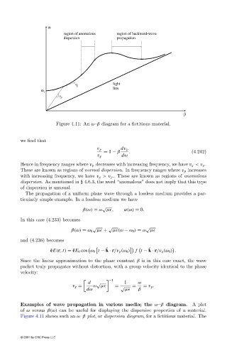
Figure 4.11: An ω–β diagram for a fictitious material.

we find that

v p dv p
= 1 − β . (4.242)
v g dω
Hence in frequency ranges where v p decreases with increasing frequency, we have v g <v p .
These are known as regions of normal dispersion. In frequency ranges where v p increases
with increasing frequency, we have v g >v p . These are known as regions of anomalous
dispersion. As mentioned in § 4.6.3, the word “anomalous” does not imply that this type
of dispersion is unusual.
The propagation of a uniform plane wave through a lossless medium provides a par-
ticularly simple example. In a lossless medium we have
√
β(ω) = ω µ , α(ω) = 0.

In this case (4.233) becomes
√ √ √
β(ω) = ω 0 µ + µ (ω − ω 0 ) = ω µ
and (4.236) becomes
ˆ
ˆ

ˆ eE(r, t) = ˆ eE 0 cos ω 0 t − k · r/v p (ω 0 ) f t − k · r/v g (ω 0 ) .
Since the linear approximation to the phase constant β is in this case exact, the wave
packet truly propagates without distortion, with a group velocity identical to the phase
velocity:

d √ 1 ω

−1
v g = ω µ = √ = = v p .
dω µ β
Examples of wave propagation in various media; the ω–β diagram. A plot
of ω versus β(ω) can be useful for displaying the dispersive properties of a material.
Figure 4.11 shows such an ω–β plot, or dispersion diagram, for a fictitious material. The

© 2001 by CRC Press LLC