Page 277 - Electromagnetics

200
180
ε
160 0 i
140 Light Line: ε=ε
ω/2≠ (GHz) 120

100
80

60 Light Line: ε=ε ε
0 s
40

20
0
0 1000 2000 3000 4000 5000 6000 7000 8000 9000 10000
β (r/m)

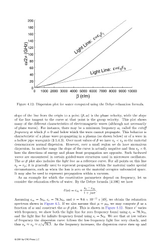
Figure 4.12: Dispersion plot for water computed using the Debye relaxation formula.

slope of the line from the origin to a point (β, ω) is the phase velocity, while the slope
of the line tangent to the curve at that point is the group velocity. This plot shows
many of the different characteristics of electromagnetic waves (although not necessarily
of plane waves). For instance, there may be a minimum frequency ω c called the cutoff
frequency at which β = 0 and below which the wave cannot propagate. This behavior is
characteristic of a plane wave propagating in a plasma (as shown below) or of a wave in
a hollow pipe waveguide (§ 5.4.3). Over most values of β we have v g <v p so the material
demonstrates normal dispersion. However, over a small region we do have anomalous
dispersion. In another range the slope of the curve is actually negative and thus v g < 0;
here the directions of energy and phase front propagation are opposite. Such backward
waves are encountered in certain guided-wave structures used in microwave oscillators.
The ω–β plot also includes the light line as a reference curve. For all points on this line
v g = v p ; it is generally used to represent propagation within the material under special
circumstances, such as when the loss is zero or the material occupies unbounded space.
It may also be used to represent propagation within a vacuum.
As an example for which the constitutive parameters depend on frequency, let us
consider the relaxation effects of water. By the Debye formula (4.106) we have

s − ∞
˜ (ω) = ∞ + .
1 + jωτ
Assuming ∞ = 5 0 , s = 78.3 0 , and τ = 9.6 × 10 −12 s [49], we obtain the relaxation
spectrum shown in Figure 4.5. If we also assume that µ = µ 0 , we may compute β as a
function of ω and construct the ω–β plot. This is shown in Figure 4.12. Since varies

with frequency, we show both the light line for zero frequency found using s = 78.3 0 ,
and the light line for infinite frequency found using i = 5 0 . We see that at low values
of frequency the dispersion curve follows the low-frequency light line very closely, and
√
thus v p ≈ v g ≈ c/ 78.3. As the frequency increases, the dispersion curve rises up and

© 2001 by CRC Press LLC