Page 339 - Electromagnetics

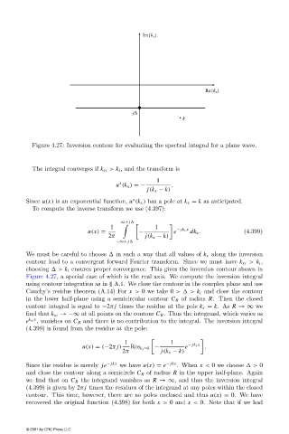
Figure 4.27: Inversion contour for evaluating the spectral integral for a plane wave.

The integral converges if k xi > k i , and the transform is

1
x
u (k x ) =− .
j(k x − k)
x
Since u(x) is an exponential function, u (k x ) has a pole at k x = k as anticipated.
To compute the inverse transform we use (4.397):
∞+ j
1 1 − jk x x
u(x) = − e dk x . (4.399)
2π j(k x − k)
−∞+ j
We must be careful to choose in such a way that all values of k x along the inversion
contour lead to a convergent forward Fourier transform. Since we must have k xi > k i ,
choosing > k i ensures proper convergence. This gives the inversion contour shown in
Figure 4.27, a special case of which is the real axis. We compute the inversion integral
using contour integration as in § A.1. We close the contour in the complex plane and use
Cauchy’s residue theorem (A.14) For x > 0 we take 0 > > k i and close the contour
in the lower half-plane using a semicircular contour C R of radius R. Then the closed
contour integral is equal to −2π j times the residue at the pole k x = k.As R →∞ we
find that k xi →−∞ at all points on the contour C R . Thus the integrand, which varies as
e k xi x , vanishes on C R and there is no contribution to the integral. The inversion integral
(4.399) is found from the residue at the pole:

1 1 − jk x x
u(x) = (−2π j) Res k x =k − e .
2π j(k x − k)

Since the residue is merely je − jkx we have u(x) = e − jkx . When x < 0 we choose > 0
and close the contour along a semicircle C R of radius R in the upper half-plane. Again
we find that on C R the integrand vanishes as R →∞, and thus the inversion integral
(4.399) is given by 2π j times the residues of the integrand at any poles within the closed
contour. This time, however, there are no poles enclosed and thus u(x) = 0. We have
recovered the original function (4.398) for both x > 0 and x < 0. Note that if we had

© 2001 by CRC Press LLC