Page 341 - Electromagnetics

2
2
2
2
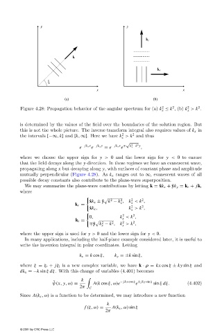
Figure 4.28: Propagation behavior of the angular spectrum for (a) k ≤ k ,(b) k > k .
x x
is determined by the values of the field over the boundaries of the solution region. But
this is not the whole picture. The inverse transform integral also requires values of k x in
2
2
the intervals [−∞, k] and [k, ∞]. Here we have k > k and thus
x
√
2
2
e − jk x x − jk y y = e − jk x x ∓ k x −k y ,
e
e
where we choose the upper sign for y > 0 and the lower sign for y < 0 to ensure
that the field decays along the y-direction. In these regimes we have an evanescent wave,
propagating along x but decaying along y, with surfaces of constant phase and amplitude
mutually perpendicular (Figure 4.28). As k x ranges out to ∞, evanescent waves of all
possible decay constants also contribute to the plane-wave superposition.
We may summarize the plane-wave contributions by letting k = ˆ xk x + ˆ yk y = k r + jk i
where

2 2 2 2
ˆ xk x ± ˆ y k − k , k < k ,
x
x
k r =
2
2
ˆ xk x , k > k ,
x
2 2
0, k < k ,
x
k i =
2
2
2
2
∓ˆ y k − k , k > k ,
x x
where the upper sign is used for y > 0 and the lower sign for y < 0.
In many applications, including the half-plane example considered later, it is useful to
write the inversion integral in polar coordinates. Letting
k x = k cos ξ, k y =±k sin ξ,
where ξ = ξ r + jξ i is a new complex variable, we have k · ρ = kx cos ξ ± ky sin ξ and
dk x =−k sin ξ dξ. With this change of variables (4.401) becomes
k
˜ − jkx cos ξ ± jky sin ξ
ψ(x, y,ω) = A(k cos ξ, ω)e e sin ξ dξ. (4.402)
2π C
Since A(k x ,ω) is a function to be determined, we may introduce a new function
k
f (ξ, ω) = A(k x ,ω) sin ξ
2π
© 2001 by CRC Press LLC