Page 342 - Electromagnetics

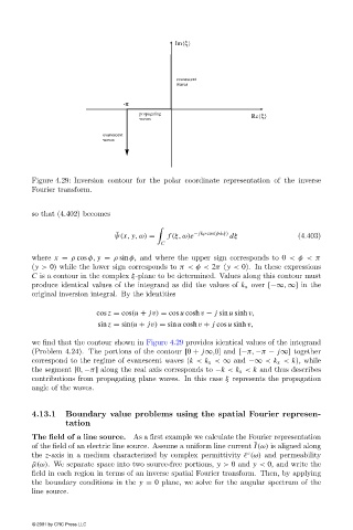
Figure 4.29: Inversion contour for the polar coordinate representation of the inverse
Fourier transform.

so that (4.402) becomes

˜ − jkρ cos(φ±ξ)
ψ(x, y,ω) = f (ξ, ω)e dξ (4.403)
C
where x = ρ cos φ, y = ρ sin φ, and where the upper sign corresponds to 0 <φ <π
(y > 0) while the lower sign corresponds to π< φ < 2π (y < 0). In these expressions
C is a contour in the complex ξ-plane to be determined. Values along this contour must
produce identical values of the integrand as did the values of k x over [−∞, ∞] in the
original inversion integral. By the identities

cos z = cos(u + jv) = cos u cosh v − j sin u sinh v,
sin z = sin(u + jv) = sin u cosh v + j cos u sinh v,

we find that the contour shown in Figure 4.29 provides identical values of the integrand
(Problem 4.24). The portions of the contour [0 + j∞,0] and [−π, −π − j∞] together
correspond to the regime of evanescent waves (k < k x < ∞ and −∞ < k x < k), while
the segment [0, −π] along the real axis corresponds to −k < k x < k and thus describes
contributions from propagating plane waves. In this case ξ represents the propagation
angle of the waves.

4.13.1 Boundary value problems using the spatial Fourier represen-
tation
The field of a line source. As a first example we calculate the Fourier representation
˜
of the field of an electric line source. Assume a uniform line current I(ω) is aligned along
c
the z-axis in a medium characterized by complex permittivity ˜ (ω) and permeability
˜ µ(ω). We separate space into two source-free portions, y > 0 and y < 0, and write the
field in each region in terms of an inverse spatial Fourier transform. Then, by applying
the boundary conditions in the y = 0 plane, we solve for the angular spectrum of the
line source.

© 2001 by CRC Press LLC