Page 345 - Electromagnetics

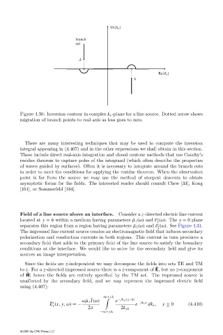
Figure 4.30: Inversion contour in complex k x -plane for a line source. Dotted arrow shows
migration of branch points to real axis as loss goes to zero.

There are many interesting techniques that may be used to compute the inversion
integral appearing in (4.407) and in the other expressions we shall obtain in this section.
These include direct real-axis integration and closed contour methods that use Cauchy’s
residue theorem to capture poles of the integrand (which often describe the properties
of waves guided by surfaces). Often it is necessary to integrate around the branch cuts
in order to meet the conditions for applying the residue theorem. When the observation
point is far from the source we may use the method of steepest descents to obtain
asymptotic forms for the fields. The interested reader should consult Chew [33], Kong
[101], or Sommerfeld [184].

Field of a line source above an interface. Consider a z-directed electric line current
c
located at y = h within a medium having parameters ˜µ 1 (ω) and ˜ (ω). The y = 0 plane
1
c
separates this region from a region having parameters ˜µ 2 (ω) and ˜ (ω). See Figure 4.31.
2
The impressed line current source creates an electromagnetic field that induces secondary
polarization and conduction currents in both regions. This current in turn produces a
secondary field that adds to the primary field of the line source to satisfy the boundary
conditions at the interface. We would like to solve for the secondary field and give its
sources an image interpretation.
Since the fields are z-independent we may decompose the fields into sets TE and TM
˜
to z. For a z-directed impressed source there is a z-component of E, but no z-component
˜
of H; hence the fields are entirely specified by the TM set. The impressed source is
unaffected by the secondary field, and we may represent the impressed electric field
using (4.407):

∞+ j
˜
ω ˜µ 1 I(ω) e − jk y1 |y−h|
˜ i − jk x x
E (x, y,ω) =− e dk x , y ≥ 0 (4.410)
z
2π 2k y1
−∞+ j
© 2001 by CRC Press LLC